Send us a message or schedule an online review to speak with a broker who’ll answer questions and provide supporting links for additional information and/or verification.
For beginners see this trade, for more advanced traders see the links below.
1) Tracking these trades and/or experimenting with any potential outcome for them.
100.0000 Represents a rate of 0.0000% (100.0000 – price = rate) -99.1650 Subtract the contract entry price 0.8350% = Markets anticipated rate for Dec. 2018 delivery at entry
100.0000 Represents a rate of 0.0000% (100.0000 – price = rate) -97.9000 Price at the lowest anticipated rate by the Fed by Dec 2018 2.1000% = Thelowest anticipated rate by the Fed for December 2018 delivery
We’re short, positioned to capture the move lower in the ZQZ18’s contract price from 99.1650 to 97.9000. This represents an increase in the Fed Funds rate from 0.8350% to 2.1000%, the the lowest of the Federal Reserve’s expectations for this rate by the end of December 2018.
5) Lowest of Fed expectations for rate hikes through 2019. (June 2017)
6) Median Fed expectations for rate hikes through 2019 (December 2014) however the Fed has been wrong on nearly every economic forecast and literally every rate call since 2008. The standard joke is the Fed no longer stands for Federal Reserve but failed economic policy.
9) Open an accountfor minimums of 10K to 500K USD or major currency equivalent, for account greater than 500K you can work with the majority of the firms listed on this page.
If you’d like to review this and/or other programs/markets please contact us or schedule an online review using this link, we’ll answer all your questions and provide you supporting links for additional information and/or verification.
If you’re stubborn about holding Treasurieswith the pending rate hikeand you or your manager doesn’t hedge downside risk you’ll have no one to blame but yourself.
Using an option collar provides protection by selling a call option against your position and using the collected premium to purchase a put option to define downside risk.
1) Benefits
Risk is defined on the trade and for the duration of the trading period
Loses will be limited when the Fed finally engages with rate hikes
If the market stays the same you’ve collected approximately as much time premium as you’ve purchased
To determine realistic risk reward levels consistent with the duration of the trade. In this example I’m trading the September 10 Year which goes off the board 21, August 2015 or 18 days from the 3 August 2015 entry.
Sell the 128 32/64th call against the long position collecting $335.94
Using the collected premium buy the 126 32/64th put paying $298.06
5) To experiment with any potential outcome for this trade
Click here to open the corresponding risk/reward spreadsheet, enable it, enter any price into cell C-2
6) Worst case scenario
Rates skyrocket, Treasuries sell off hard to 110 0/32nds for a loss in contract value of -17,812.50 or – 13.93% but because we’re hedged our loss was limited to -$1,266
7) To confirm
A) Enter 110 0/32 in cell C-2
B) Net loss shows in cell E-2
C) Net liquidating value shows in cell E-3
8) The market stays the same you’ve collected your credit premium of $47 plus your interest income.
A) Enter 127 26/32nds in cell C-2
B) Net loss shows in cell E-2
C) Net liquidating value shows in cell E-3
9) Rates move lower, Treasuries rally, the position is called away at a $734 profit plus your interest income and we can reestablish the position immediately.
A) Enter 2,000 in cell C-2
B) Net loss shows in cell E-2
C) Net liquidating value shows in cell E-3
For more advance traders we can write a put below the market for reentry where the only way we could be delivered a position is at a better price, if the market never goes down to the strike we keep the premium.
Example the 127 put is nearly a full point below the market with a time decay of 0.06% per month or 7.24% annually (far more than the interest income)
If delivered a position you can collar it explained above
Or
You can write a call above the market for example 128 16/32 collecting 0.07% per month or 8.5% annually ,the only way the position can be called away from you is at a profit 0.54% or you were paid 0.7% for that month to sell it at a profit (in at 127 26/32nds out at 128 12/32nds).
Using this strategy the worst thing that will happen to you is you would own a bond that you would have bought or already owned anyway.
Contact me for more information on yield enhancement
These strategies can be traded in any liquid market, crude oil and grains have the highest premium currently relative to contract value.
An option option collar provides defined risk on a long or a short position by selling an option against your position and using the collected premium to purchase an option to protect your position to objectively define risk
1) Benefits
Risk is defined on the trade and for the duration of the trading period
The position cannot be stopped out
If the market stays the same you’ve collected approximately as much time premium as you’ve purchased
The only way the position can be called away is at a profit
2) Identify the current trend using a daily chart, the red red line exponential moving average 9 (EMA9) above the blue line (EMA18) trade long Red EMA9 below blue EMA18 trade short
Red EMA9 is below the Blue EMA 18, the S&P ready for a correction, establish your position with the trend.
Determine realistic risk reward levels consistent with the duration of the trade. In this example I’m trading the September S&P which goes off the board 18 September 2015 or 46 days from our 3 August 2015 entry.
PROGRAM AVAILABILITY IS DEPENDENT ON YOUR COUNTRY OF RESIDENCY AND FINANCIAL STATUS
PAST RESULTS ARE NOT NECESSARILY INDICATIVE OF FUTURE RESULTS. EXAMPLES OF HISTORIC PRICE MOVES OR EXTREME MARKET CONDITIONS ARE NOT MEANT TO IMPLY THAT SUCH MOVES OR CONDITIONS ARE COMMON OCCURRENCES OR ARE LIKELY TO OCCUR.
HYPOTHETICAL PERFORMANCE RESULTS HAVE MANY INHERENT LIMITATIONS, SOME OF WHICH ARE DESCRIBED BELOW. NO REPRESENTATION IS BEING MADE THAT ANY ACCOUNT WILL OR IS LIKELY TO ACHIEVE PROFITS OR LOSSES SIMILAR TO THOSE SHOWN IN FACT, THERE ARE FREQUENTLY SHARP DIFFERENCES BETWEEN HYPOTHETICAL PERFORMANCE RESULTS AND THE ACTUAL RESULTS SUBSEQUENTLY ACHIEVED BY ANY PARTICULAR TRADING PROGRAM. ONE OF THE LIMITATIONS OF HYPOTHETICAL PERFORMANCE RESULTS IS THAT THEY ARE GENERALLY PREPARED WITH THE BENEFIT OF HINDSIGHT.
IN ADDITION, HYPOTHETICAL TRADING DOES NOT INVOLVE FINANCIAL RISK, AND NO HYPOTHETICAL TRADING RECORD CAN COMPLETELY ACCOUNT FOR THE IMPACT OF FINANCIAL RISK IN ACTUAL TRADING. FOR EXAMPLE, THE ABILITY TO WITHSTAND LOSSES OR TO ADHERE TO A PARTICULAR TRADING PROGRAM IN SPITE OF TRADING LOSSES ARE MATERIAL POINTS WHICH CAN ALSO ADVERSELY AFFECT ACTUAL TRADING RESULTS. THERE ARE NUMEROUS OTHER FACTORS RELATED TO THE MARKETS IN GENERAL OR TO THE IMPLEMENTATION OF ANY SPECIFIC TRADE PROGRAM WHICH CANNOT BE FULLY ACCOUNTED FOR IN THE PREPARATION OF THE HYPOTHETICAL PERFORMANCE RESULTS AND ALL OF WHICH CAN ADVERSELY AFFECT ACTUAL TRADING RESULTS.
BID/ASK SPREADS, BROKERAGE COMMISSION, CLEARING, EXCHANGE AND REGULATORY FEES WILL HAVE AN ADVERSE IMPACT ON THE NET OVERALL PERFORMANCE OF YOUR ACCOUNT. PRIOR TO MAKING A DECISION TO PARTICIPATE IN ANY INVESTMENT MAKE SURE YOU FULLY UNDERSTAND THE FEES ASSOCIATED WITH TRADING.
THE INFORMATION PROVIDED IN THIS REPORT CONTAINS RESEARCH, MARKET COMMENTARY AND TRADE RECOMMENDATIONS. YOU MAY BE SOLICITED FOR AN ACCOUNT BY ONE OF OUR REPRESENTATIVES OR EMPLOYEES. IT SHOULD BE KNOWN THAT THE REPRESENTATIVES OF OUR FIRM MAY TRADE FUTURES AND OPTIONS FOR THEIR OWN ACCOUNTS OR THOSE OF OTHERS. DUE TO VARIOUS FACTORS (SUCH AS MARGIN REQUIREMENTS, RISK FACTORS, TRADING OBJECTIVES, TRADING INSTRUCTIONS, TRADING STRATEGIES, AND OTHER FACTORS) SUCH TRADING MAY RESULT IN THE LIQUIDATION OR INITIATION OF FUTURES OR OPTIONS POSITIONS THAT DIFFER FROM THE OPINIONS AND RECOMMENDATIONS FOUND IN THIS REPORT.
PAST PERFORMANCE IS NOT NECESSARILY INDICATIVE OF FUTURE PERFORMANCE. THE RISK OF LOSS IN TRADING FUTURES CONTRACTS OR COMMODITY OPTIONS CAN BE SUBSTANTIAL, AND THEREFORE INVESTORS SHOULD UNDERSTAND THE RISKS INVOLVED IN TAKING LEVERAGED POSITIONS AND MUST ASSUME RESPONSIBILITY FOR THE RISKS ASSOCIATED WITH SUCH INVESTMENTS AND FOR THEIR RESULTS.
YOU SHOULD CAREFULLY CONSIDER WHETHER SUCH TRADING IS SUITABLE FOR YOU IN LIGHT OF YOUR CIRCUMSTANCES AND FINANCIAL RESOURCES.
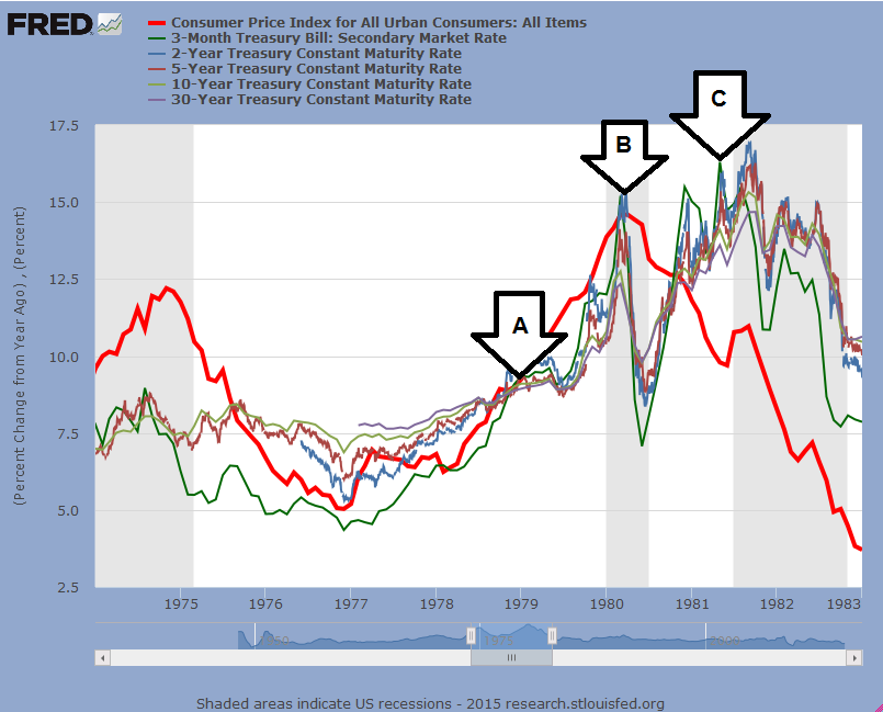
2) If you’re in the 8% minority that believe the BLS.GOV CPI calculations are correct the average annual CPI during the “Great Recession” has been 1.58%
3) If you are in the 92% that currently do not give BLS.GOV inflation numbers creditability you’re supported by actual increases.
4) 1980 and 1990 inflation calculations also support the 92%
5) Click here for current charts and more information on 1980 & 1990 CPI calculations.
Using 1980 BLS.GOV calculation methods the inflation rate would be greater than 7.50%
6) Using 1990 BLS.GOV calculations the inflation rate would be near 4.00%
By the BLS.GOV massaging the CPI lower (as they have through their current revisions and “enhanced calculation methods”) the BLS.GOV has saved the .GOV trillions in debt service costs and reduced all other cost increases that are tied to inflation.
7) Where rates should be using current BLS.GOV inflation calculations if you are in the 8% minority that give them creditability.
The 40 year average for Treasury yields is 2.14% above the CPI, the current average Treasury rate is 2.37%
Click here for the current Fed chart and supporting historical data
8) If yields went back in line with the 40 year average above the CPI Treasury yields would increase from 2.37% to 3.72% for an increase in debt service cost from the current 430 billion to 675 billion annually
Debt service cost alone would consume 36% of total U.S. annual US tax receipts.
9) Where rates would be relative to historical averages
If yields went back in line with their 40 year average the average Treasury rate would increase from 2.37% to 6.14%. Debt service cost would increase from 430 billion annually to 1.117 trillion consuming 64% of all annual tax receipts.
Where rates would be using 1980 BLS.gov calculation methods for the CPI
The current CPI using 1980 calculations would currently be 7.57%.
Using the historical average Treasury yield above the CPI Treasury the average Treasury yield would rise to 9.71% increasing the debt service cost from 430 billion to 1.77 trillion consuming 97.25% of total US tax receipts.
Can you see why the BLS.GOV needs to massage the CPI numbers lower to bailout their parent company the .GOV?
10) Pre BLS.GOV revision magic
The CPI in orange, debt in red, M1 in blue and tax receipts in green all move together.
Click here for the Fed chart and supporting historical data
11) Post BLS.GOV revision magic
You don’t have to be a Rhodes scholar to come to the conclusion the BLS.GOV’s inflation numbers would justify a name change for BLS.GOV to just BS.GOV. Click here for the current Fed chart and supporting historical data
12) During the “Great Recession” and “Economic Stimulus” the U.S achieved the worst credit rating and debt to GDP ratio in history.
Click here for the current Fed chart and all supporting historical data
13) The worst debt to tax receipt ratio in history
Click herefor the current Fed chart and all supporting historical data
14) The worst debt to disposable income ratio in history
Click here for the current Fed chart and all supporting historical data
15) The worst debt to the employed population ratio in history.
Click here for the current Fed chart and all supporting historical data
16) The worst debt to hourly earnings ratio in history
Click here for the current Fed chart and all supporting historical data
17) The worst debt to the dollar index ratio in history
Click here for the current Fed chart and all supporting historical data
18) Nearly every ratio is far worse than pre “economic stimulus”
Many including myself believe “economic stimulus” has created a far greater problem for the U.S. economy than the one it was designed to solve.
19) Why rates will rise
What everyone seems to forget up until 2008 the market basically controlled Treasury rates not the Fed.
When a country like the US needed money to finance deficit spending it created debt instruments that were sold at auction with the buyers setting the rate at auctions based on a country’s debt rating, creditability and economic outlook.
From 2008-2014 the Fed created trillions of dollars backed by no tangible assets or income flow the buy the majority of all new issues (up to 85 billion per month) to force and hold rates at artificial and unsustainable lows (Quantitative Easing)
21) This essentially shut down free market Treasury auctions and the free market determining a fair rate.
Click here for the current Fed chart and all supporting historical data
22) To put this into proper perspective 85 billion per month is 1.020 trillion annually or an amount more than twice the national debt in 1971 the year the US abandoned the Gold Standard.
Click here for the current Fed chart and all supporting historical data
23) Buy forcing rates to artificial lows the Fed created the largest negative rates of return for the longest period of time in history for holders of US debt..
Fed policy striped these “savers” and the free market economy out of trillions of dollars to save the U.S. Treasury the same amount in debt service cost, note the yields below the CPI during “economic stimulus” = a negative rate of return.
Click here for the current Fed chart and all supporting historical price data
24) Meanwhile banks never lowered the prime from 3.25%, the same banks that created the problem were allowed to lock in the largest profit margins on their borrowing costs in history for the longest period of time in history, note the Fed Funds borrowing rate relative to the prime rate the spread is 3.15% or more than 50% higher than the historical average of 2.00%.
Click here for the Fed chart and all supporting historical data
25) The Fed’s theory was to increase money supply, lie about inflation (with the help of BLS.GOV) and helicopter Ben Bernanke would inflate the U.S out of the recession back into artificial and unsustainable prosperity.
Bernanke outlines what his game plan was well before he became the chairperson of the Federal Reserve in this speech “Deflation Making Sure It Doesn’t Happen Here”
26)Click herefor this speech posted on the Fed’s website.
2& His unproven theory was/is there is a direct correlation between the increase in M1 and tax receipts which is as true, inflation engages, prices of goods and services rise with it tax revenue.
Click here for the current Fed chart and all supporting historical data
28) What Ben didn’t take into account was the ability of U.S. politicians to outspend true inflation and tax receipt increases.
Click here for the current Fed chart and all supporting data
29) Nor did he take into account the the banking problems we’re slightly larger the TARP (700 billion) when CBS and Bloomberg were able to obtain the true figures through the Freedom of information act the total exceeded 7.7 trillion
30) Nor was his team prepared or honest
Rep. Alan Grayson questions the Fed inspector General where $9 trillion dollars went… the Fed inspector general elizabeth coleman didn’t have a clue or was it the 5th?
31) But being wrong and/or incompetent was nothing new to Ben Shalom Bernanke, B,S. Bernanke was consistently wrong on his calls on the economy before and after he became Fed chairman.
Click here for the video of his calls and the outcome
32) How U.S. “leaders” could let him orchestrate an unaudited, undisclosed mult-trillion dollar “economic stimulus” plan with his proven track record for failure is beyond me.
Economic stimulus did save the U.S. Treasury trillions in debt service costs at the expense of savers.
It did make banks trillions in inflated borrowing costs at the expense of borrowers.
It did increase the per capita portion of the national debt for every American taxpayer from 67K to over 130K.
33) Now without the Fed creating trillions of dollars with keypunch entries to buy the majority of US debt at non competitive prices who’s going to replace the Fed?
Click here for the current chart and all supporting historical data
34) If the Fed fires up the QE printing press again US creditability will deteriorate even further potentially leading to 6 trillion in foreign held US debt being sold off.
Click here for the current Fed chart and all supporting historical data
35) USD currency risk for these foreign investors is more in one day than annual yields
The dollar is near a 10 year high and the world is questioning if the USD truly is the least worst place to be?
Click here for the Fed chart and all supporting historical data
36) Would you buy a U.S. Treasury with current currency risk at the rates below?
37) China’s currency is also on deck to be the world’s 5th world reserve currency and their numbers according to the Fed are far superior to the US’s
38) Click here for China versus the US using the Fed’s numbers
39) From historic lows near zero what is the only direction short term rates can have a major market move?
Click here for the current chart and all supporting historical data
40) Rates will rise from either economic recovery or deteriorating U.S creditability the only question that remains is when.
41) Fed chair Yellen has spelled out where the Fed expects rates and when on multiple occasions over the last year,
Call if you have questions, need additional information, or wold like to do a 15 minute online review where I’ll show you exactly what we’re trading and how using actual trades.
When our review is complete you’ll be able to experiment with any potential outcome for these trades or your own risk/reward criteria.
2) Fed’s expectations for the rate they set and contract valuations
0.12% contract value = $500.00 (November 2015) 1.97% contract value = $8,208.33 (13 June 2018)
2.40% December 2018 = $10,000.00
3.10% December 2019 = $12,916.67 3.40% December 2020 = $14,166.67 Each 0.01 = $41.67
Entry = 0.8350 value $3,479.17 to Fed Objective 3.40 value $14,166.65
5.1) Entry short ZQZ18 99.1650 (3 October 2016)
Rate the contract price represents 100.0000 – 99.1650 = 0.8350%
Contract value = 0.8350 X $4,166.67 = $3,479.17
5.2) At Fed’s Objective 100.0000 – 3.40 = 99.6000
Rate the contract price represents 100.0000 – 99.6000 = 3.4000%
Contract value = 3.4000 X $4,166.67 = $14,166.65
Gain if the Fed is correct = +$10,687.48
This position will need to be rolled December 2018
Current chart updated every 5 minutes, each 0.01 = $41.67
6) Trading 3 month deposits outside the Treasury System (eurodollars)
7) Trading the rate hikes between September 2018 and December 2020
Entry = 0.39 value $3,900 to the Fed’s Objective 1.40 value $14,000
7.1) Entry the 29th of May 2018
Long 4 December 2018 GEU18 97.6350
Short 4 December 2020 GEZ20 – 97.2450 IntraMarket Spread GEZ18 97.6350 – GEZ20 97.2450 = 0.39
Market’s expected rate hike between Sep. 2018 & Dec. 2020 = 0.39% Entry position value = 0.3900 X $10,000.00 = $3,900.00
7.2) Our Objective is the Fed’s Target Fed’s expected rate hikes by December 2020 = 1.40
Position value at the Fed’s target, 1.40 X $10,000.00 = $14,000.00 (The nearby delivery will have to be “rolled” quarterly) 7 year spread chart GEU18 – GEZ20
Strategy: I’m using split objectives on this trade, 1/2 of the position (2 contracts) in at 0.40 or better out at 0.55 to 0.75. 1/2 (2 contracts) trading long-term from 0.3150 to the objective of 1.40 or until we have to roll the GEU18 or the major trend reverses.
8) Trading Rate hikes between December 2018 and December 2020
8.1) Entry the 29th of May 2018
Long 4 December 2018 GEZ18 97.4200
Short 4 December 2020 GEZ20 – 97.1050 IntraMarket Spread GEZ18 97.42 – GEZ20 97.1050 = 0.3150
Market’s expected rate hike between Dec. 2018 & Dec. 2020 = 0.3150%”
Position value 0.3150 X $10,000.00 = $3,150.00 Spread chart GEZ18 – GEZ20 in at 0.3150 expecting the price to increase Complete report on this trade
8.2) Minimum Objective 0.65 Position value at 0.3150 entry = $3,150.00
Position value at the minimum objective of 0.65 = $6,500 Gain = $3,350 (106.34%) Spread chart GEZ18 – GEZ20
8.3) At the Fed’s 1.00 target Position value at 0.3150 entry = $3,150.00 Position value at the Fed’s target of 1.00 = $10,000.00
Gain = $6,850.00 (217.45%) Spread chart GEZ18 – GEZ20
Current chart updated every 5 minutes, each 0.01 = $100.00
Strategy: I’m using split objectives on this trade, 1/2 of the position (2 contracts) in at 0.40 or better out at 0.55 to 0.65. 1/2 (2 contracts) trading long-term from 0.3150 to the objective of 1.10 or until we have to roll the GEZ18 or the major trend reverses.
9) Trading Rate hikes between September 2018 and December 2023
9.1) Entry the 31th of May 2018
Long 4 September 2018 GEU18 97.5650
Short 4 December 2023 GEU23– 96.9950 Intramarket Spread GEU18 (97.5650) – GEZ23 (96.9950) =0.5750% Market’s expected rate hike between Sep. 2018 & Dec. 2023 = 0.5750%
Position value 0.5750 X $10,000.00 = $5,750.00 Spread chart GEZ18 – GEZ23 in at 0.5750 expecting the price to increase
9.2) Minimum Objective 1.00 Position value at 0.5750 entry =$5,750.00
Position value at the minimum objective of 1.00 = $10,000.00 Gain = $4,250.00 (73.91%) Spread chart GEZ18 – GEZ23
9.3) Our Long Term Objective 2.10 Position value at 0.5750 entry = $5,750.00 Position value at the objective 2.10 = $21,000.00
Gain = $15,250.00 (265.21%) Spread chart GEZ18 – GEZ23
Current chart updated every 30 minutes, each 0.01 = $100.00
Strategy: I’m using split objectives on this trade, 1/2 of the position (2 contracts) in at 0.60 or better out at 0.75 to 0.90. 1/2 (2 contracts) trading long-term from 0.5750 to the objective of 2.10 or until we have to roll the GEU18 or the major trend reverses.
10) If you’d like to track additional positionssend me message
Prior to the sell off in housing Bernanke assures everyone housing prices will be steady to higher, there is no bubble, home prices will be supported by the strength in the economy and “there has never been a national decline in home prices”.
8) Bernanke’s call = Moderate growth in the economy moving forward
Gross Domestic product contracts beyond the worst of analysts expectations
Click here for the Fed Gross Domestic Product chart
9) Bernanke’s call = The sub prime mortgage market is healthy and liquid
One year latter over 50 of the largest investment banks fail, declare bankruptcy or are acquired because of illiquid failed mortgages. The US has the highest mortgage delinquency rate on record.
This is one of 900+ speeches Bernanke has given where the majority of his calls on the economy have been notoriously bad.
The US is now faced the worst financial crisis since the Great Depression.
With his record of failure Washington still allows him craft the largest and most costly “economic stimulus” program in US history enabling him to direct unaudited amounts of money that exceed the US GDP.
11) Bernanke’s “economic stimulus” engages
The Fed creates trillions to force and hold rates at artificial and historic lows.
Federal debt in red, interest paid in green, Fed purchases of US debt in bright blue
12) Low rates strip savers of over ½ a trillion in interest income annually.
Savers are forced to endure the largest negative rates of return for the longest period in history. This 1/2 trillion is stripped from the free market economy to save the U.S. Treasury the same amount in debt service cost.
While savers are being striped of over 1/2 a trillion in interest income the Fed creates nearly 8 trillion with keypunch entries from 2007 to 2009 to bail out the same banks that created the crisis. Source CBS, Bloomberg and the freedom of information act, again the Fed created this money with keypunch entries.
13) Bailouts by the numbers video
14) Fed’s Inspector General clueless about 9 trillion?
Rep. Alan Grayson questions the Fed inspector General where $9 trillion dollars went… the fed inspector general elizabeth coleman didn’t have a clue.
15) In 2009 the Fed moves from bailouts to outright purchases of 1.7 trillion of bad loans to bail out the same banks that created them.
U.S. Banks never lowered the prime, it has remained unchanged at 3.25% since 2009 locking in the largest gross bank profit margins on borrowing costs for the longest period of time in history.
The 1954-2015 average spread between Fed funds (bank borrowing rate) and prime is 2.00% during economic “stimulus” is has averaged 3.15% or over 150% of the historical average. Not that the Japanese are an act to follow but at least they had the conscience to lower their prime to 1.20%.
If the Fed funds rate rose by 1.00% and the prime remained constant at 3.25% the spread between Fed funds and prime would still be larger than the 1954-2015 historical average of 2.00%
Through the creation of money backed by no tangible asset or income flow the Fed believes the prices of goods and services will rise, with it tax revenue allowing the U.S to exchange its governmental and bank debt problems for inflation and economic recovery with tax revenue outpacing inflation. Click here for his speech.
One thing Bernanke did not anticipate which had already been proven was the ability of government to out spend monetization and currency devaluation.
18) Once again the US proved the monetization theory wrong
3 other countries with world currency status Japan, the European Union and the UK also entered the same monetization race to exchange their debt problems for inflation problems.
With all four world currencies working together they give the impression the 4 world reserve currencies are somewhat stable against each other but not against tangible assets like gold.
The the USD, JPY, EUR and GBP have been hammered against gold but because they have declined together it appears they are somewhat stable.
At the same time these countries have adopted inflation calculation methods which give give the appearance inflation is contained when in reality it’s 2 to 3 times the reported numbers to justify low rates and contain increases in governmental programs.
Gold tells the true story about coordinated currency devaluation but appears to be the aberration. Click herefor more on inflation calculation magic.
Increase in the national debt since the U.S. went off the gold standard = 4,4562% Increase in the price of goldsince the U.S. went off the gold standard = 3,2855%
M1 has expanded, tax tax receipts and home prices have increased with it while the Bureau of Labor and Statics (BLS.gov) did their “adjustment magic” to keep official inflation low justifying low rates. The harsh reality is people in the US are working longer now to buy the same goods and services than at the height of the Great Depression in 1933.
20) Longer Term Results of Bernanke’s Failed Multi Trillion Dollar Experiment.
Debt to tax receipts have disabled the US from servicing it’s debt, each 1% increase in rates consumes 10% of all tax receipts.
The last time the U.S. raised rates (June 2006)
Federal debt = 8.4 trillion Tax receipts = 1.40 trillion US debt as a percentage of GDP = 61%
Current Federal debt = 18.1 trillion Tax receipts = 1.8 trillion US debt as a percentage of GDP = 102%
Should interest rates normalize going back to the 1954-2015 average of 5.10% nearly 50% of all tax receipts will be consumed by debt service cost alone pushing annual budget deficits close to 2 trillion dollars annually.
U.S. Taxpayers, Savers and their Children are getting a 9+ trillion dollar tab
Bernanke’sfailed “economic stimulus experiment” has increased the employed population’s per capita share of the national debt increasing from 67K to over 130K. If rates return to the 1954-2015 historical average of 5.10% debt service cost per employed U.S. worker will be $6,732 annually.
26) On deck
The US has 6 Trillion of U.S. debt that is currently owned by non U.S. investors, trillions more in stocks, muni and corporate bonds, currency risk in one day for these non US investors is more than annual yields/dividends.
27) The dollar is coming off a 10 year high and looking heavy
The Fed U.S dollar index since March 2015 has sold off from 93.10 to 87.58 or -8.077% for a loss of 526 billion on the 6 trillion owned in just US Treasury debt, 10’s of billions more on share, muni and corporate debt positions.
Click here for more Fed charts comparing China to the US.
29) Contagion exposure isn’t Greece
The move generated by the Greece June 29th and 30th does not represent “contagion” but should be a warning to all. The DAX -3.7%, FTSE -2.1%, CAC -3.8%, S&P -1.2% DOW -1.33%.
The European Union has a GDP of 18.5 trillion (USD) Greece is 242 billion representing less than 2% of the European Union’s total GDP.
To put this into perspective Greece’s GDP is just a little larger than the state of Louisiana (216 billion),
California’s GDP is 2.3 trillion and just think of how many times the State of California has nearly gone broke,
Orange county California’s GDP is 210 billion and was forced to file for bankruptcy in 1994.
If Greece on June 29th and 30th can create this DAX -3.7%, FTSE -2.1%, CAC -3.8%, S&P -1.2% DOW -1.33% just think of the damage and “global contagion” that will engage when sales of 6 trillion or foreign held U.S debt engages.
The harsh reality for the U.S. and other western economies is there monetary policy is unsustainable, and now irreversible because of prewar Germany/Bernanke style “economic stimulus” their only out now is currency devaluation and inflation, clickhere for the numbers and links to Fed charts
30) How this will unwind
1) As the dollar loses credibility foreign sales of U.S. debt, shares and dollar’s will engage
2) These sales will escalate as U.S. rates rise rise and Treasury instrument valuations fall
3) Higher rates will hurt U.S. companies resulting in U.S. stock sales
4) China’s currency comes on board as the 5th world reserve currency in October
The U.S. markets will hemorrhage, true contagion will spread to the European Union if is does not occur first in the EU giving the Fed the justification to fire up the “Quantitative Easing” printing press with a vengeance.
31) High true inflation will engage
Total debt service cost in 2014 = $430.81 billion. Average 2014 interest rate = 2.37%
32) The majority of all U.S. debt is now fixed in durations of 10+ years
Average yield on this debt is 2.37%, (1954-2015 Average 5.10%)
The U.S. has the worst economic fundamentals in it’s history
The U.S. has locked in fixed financing at 2.37% less than half the 1954-2015 average treasury yield of 5.10%
By keeping short term rates near zero those that needed any income were “sucked” into the longer dated U.S. Treasuries allowing the U.S. Treasury to lock in its debt service cost at the lowest rates in history for the longest average duration in history.
This will allow the U.S. to massively devalue the dollar with little or no impact on debt service cost as dollar devaluation and inflation engages.
The same investors who have endured the largest negative rates of return for the longest period in history now face the largest dollar and instrument devaluation in history.
33) Further Monetization now remains the only solution (devalue the dollar)
Pre Monetization interest rate risk to U.S. budget deficits
Had the U.S not “fixed” it’s debt for the next 10+ years the coming interest rate hikes could be catastrophic.
The 2008-2014 average U.S. federal deficit was 1.4506 trillion or greater then the total national debt in 1984 of 1.4107 trillion.
Yellow = current treasury rate with debt service consuming -23.41% of total tax receipts Red = 1954-2015 average Treasury rate with debt service consuming -50.28% of tax receipts Orange what rates would be using BLS.GOV calculations from 1980, -92.88% of tax receipts
34) Through the creation of money backed by nothing “Quantitative Easing” increases money supply.
As more money chases after the same goods and services prices rise (inflation).
When prices rise so does tax revenue which I believe is the Fed’s ultimate goal, to have the same debt service cost from the fixed rate with potentially twice the revenue to service it.
The Fed chart below shows the direct correlation between M1 (money supply) in black and tax receipts in green.
35) Post Monetization (after the Fed devalues the dollar against tangible assets)
U.S. Treasury debt is fixed for greater than 10 years the impact on debt service cost will be minimal with the increase in inflated tax revenue offsetting the increase in rates.
Yellow = current treasury rate with debt service consuming -11.71% of tax receipts Red = 1954-2015 average Treasury rate with debt service consuming -25.14% of tax receipts Orange what rates would be using BLS.GOV calculations from 1980, -46.44% of tax receipts
One thing no one can question is the great recession has generated extreme economic fundamentals.
Extreme economic fundamentals generate trends and the kind of markets and profit potential traders like myself dream about.
The following are the expectations for today’s FOMC June policy meeting as provided by the economists at 22 major banks along with some thoughts on the USD into the event as provided by the FX strategists at these banks.
Goldman: The overarching message from the meeting will probably be that September remains the Committee’s baseline expectation for the start of monetary tightening, reflecting cumulative progress in the recovery over the last six years. While September remains our baseline as well, we think that the FOMC will want to preserve optionality at the June meeting, and there is still a significant probability that the hiking cycle will not begin until December or later. We expect the content of the Summary of Economic Projections (SEP)—released coincident with the FOMC statement—to be updated to reflect the recent economic data. The unemployment rate path will likely be slightly higher in the near term, while long-term views on the natural rate of unemployment may come down further. Participants’ assessment of the inflation outlook will probably be little changed. Most importantly, we think that both the median and modal “dot” will remain at 0.625% for 2015, consistent with two twenty five basis point hikes this year (beginning in September). However, most other aspects of the dot plot will probably show a dovish shift, reflecting softer H1 activity and the Fed’s “data dependent” mantra.
Barclays: Markets will pay close attention to the tone of the FOMC statement on Wednesday and watch for hints on the timing of the first rate hike. Given the recent pickup in US consumption and labor market data, we think the Fed is likely to maintain its view that the winter slowdown was transitory and that the economy is likely to expand at a moderate pace. Indeed, the pace of job growth has picked up, with payrolls rising 280K in May, and the Fed’s LMCI has increased since the April meeting. Additionally, we expect the Fed to reiterate that inflation will gradually rise toward the 2% target in the medium term as the labor market continues to improve and inflation expectations remain stable. Indeed, CPI data on Thursday, along with the latest import price data, should support our view that downward pressures on domestic core inflation from the lagged effects of USD appreciation will begin to wane going into the third quarter. As such, we continue to think the Fed is on track to hike twice this year (at the September and December meetings). Overall, we believe that the FOMC statements, along with CPI and other macro data, should support the USD
UBS: We expect Chair Yellen to continue setting the stage for the start of the Fed’s tightening cycle later this year. If market expectations are correct, the June FOMC meeting will be the last quarterly update to the FOMC’s forecasts before the Fed at the September 16-17 FOMC meeting hikes rates for the first time in more than nine years. (The previous rate hike was on June 29, 2006.) As a consequence market participants are focused on the upcoming meeting despite no expectation that the Fed funds target rate will be immediately increased. We do not expect the post-meeting statement, the forecast or the press conference to prompt a rethinking of current market expectations. As of Friday the markets were pricing in a bit more than 75% chance of a rate hike at the September FOMC meeting. We believe the FOMC is currently comfortable with that view and is cognizant of the fact that there are ample opportunities to reset market expectations, if needed, before the September meeting.
Deutsche Bank: The statement should have a more positive tone, especially regarding the labor market. Our forecasts of the Fed’s central tendencies are shown in the table below. Despite a reduction in 2015 GDP, we do not believe the median 2015 fed funds dot will change. Any reduction in the median 2015 dot would immediately focus market participants’ collective attention on the December meeting, and the Fed surely wants the option to hike in September, data permitting…Regarding the press conference, Yellen will reaffirm the case for beginning the process of policy normalization sometime later this year. The Fed Chair’s May 22 speech was telling in that she subtly shifted the conversation from outlining why the Fed may begin raising interest rates to how far and how fast they may go after liftoff. She may choose to elaborate on some of the themes of that speech, including productivity growth. In short, we expect the Fed Chair to continue to de-emphasize the timing of liftoff and focus financial market participants on the factors the Fed will be taking into account in determining the pace of policy normalization.
BNP Paribas: We expect today’s FOMC statement to acknowledge improvement in key data after transitory factors suppressing Q1 activity abated. In the subsequent press conference, Chair Yellen will likely continue to emphasize that rate hikes are likely coming at some point later this year. However, the meeting may not provide a decisive catalyst for the US currency. Our economists note that the FOMC’s projection ‘dots’ are likely to shift in a dovish direction as the more hawkish members acknowledge that tightening will not begin in mid-2015. The Committee and Chair Yellen will also need to explain its decision to leave rates unchanged now and be sure to avoid signalling lift off at the July meeting. Rate markets remain underpriced relative to our expectation for tightening to begin in September but we may need to wait for more economic data and subsequent Fed communications before we see an adjustment to our view
Credit Suisse: We expect the FOMC to acknowledge the improvement in US economic statistics since the reported contraction in 1Q. But the rebound in activity is still building momentum and has not been sufficiently conclusive, in our view, to prompt the Fed to tighten policy as soon as this month. Also, while we do assign a small positive probability to a July rate hike, say 15%, we believe September to be the most likely date for policy lift-off. Various scenarios related to the June 16–17 meeting include the possibility of more explicit guidance in the policy statement on the timing of a rate hike (not likely in our view) and downward revisions to GDP growth forecasts.
Nomura: The FOMC is likely to clearly keep September lift-off on the table when it meets this week. After better data momentum, the text of the statement is likely to sound more confident, and the dots are likely to signal that a two-hike scenario in 2015 is still the central case. While one hike has again become the central case, a two-hike scenario is still priced with a fairly low probability. We think the two-hike scenario is around 60% probability, and if this is true, the short end has more room to sell off.
SocGen: The risk at this evening’s FOMC meeting is, that while the underlying economic vies are reasonably upbeat and consistent with ‘lift-off’ happening in September, the (in)famous ‘dot-path’ will be lowered enough to be the main talking point. The FOMC ‘dots’ project 2 rate hikes this year and 5 next, so a total of 1.75% in hikes by the end of 2016. The Fed Funds futures price a 1% rise in rates over the same period, and our economics team expects the dot-plot to be cut back to 125bp. Is the market going to see this as a non-event, affirmation that too little is priced in, or a dovish signal? I rather fear the last of these may win the day but all will be clearer at 19:00 BST or, more likely after 19:30 when the press conference allows Janet Yellen to send the signal she wants. Either way, the bigger move is more likely to come in July/August as data convince people that a hike is coming
Credit Agricole: We expect no changes to rates at the June FOMC meeting and continue to expect rate normalization to begin in September. No rate hikes are expected as policymakers continue to assess progress towards conditions conducive for lift-off. These include (1) continued improvement in labour market conditions and (2) reasonable confidence that inflation will move back to its 2% objective over the medium term. We believe the Fed is close to meeting its employment mandate. However, the Fed is likely to require more evidence before being reasonably confident that inflation will rise towards its 2% objective over the medium term. Assessing the transitory impacts on growth and the economy’s underlying momentum will require more time. However, we believe that the FOMC will see evidence that the conditions for lift-off have been met by the September FOMC meeting. The updated Summary of Economic Projections (SEP) will likely lower GDP growth projections for 2015 in light of the Q1 GDP contraction. We believe most Fed officials expect to begin hiking rates this year. The year-end 2016 median fed funds rate projection may come in slightly below the March projection, in line with the gradual pace of anticipated rate normalisation.
ANZ: Market focus will turn to the FOMC meeting this week and there are three areas to watch for the USD. The first is any commentary on the USD – there has been an increase in official rhetoric about the strength of the USD negatively impacting on the US of late, and this is important for the medium-term USD path. The second is economic growth projections. The market and ANZ expects the Q1 GDP weakness to lead to official 2015 growth forecasts revised lower. The final area to focus on is the ‘dot points’.
RBS: The key hawkish risk at this week’s June FOMC meeting may come from the signaling language. The April meeting minutes revealed that the Fed discussed (and opted not to) give a broader signal that rate hikes were coming soon – any direct step to “prepare” the market for a rate hike via the press conference or statement language would likely be a USD positive. With only 6-months to go before year-end, the market may put focus on the near-term FOMC “dot” projections released this week, where the median currently suggests the Fed can hike twice before year-end. No change in the dot point projections for 2015 could be seen as a positive as only one hike is priced in for the remainder of the year. The well-telegraphed sluggish start to the economy may result in a downward revision to 2015 growth forecasts, and that may leave risks to the “dot point” Fed Funds rate projections as moderately to the downside. Even so, we think the Fed sending a message about increased confidence in their positive outlook may overshadow a revised growth profile.
Lloyds: While a hike in interest rates at today’s FOMC meeting looks highly unlikely, the meeting could still provide clues about the timing of a first move. An important indication of the likelihood of a relatively early rise in rates will be the extent to which the post-meeting statement is more upbeat about recent economic developments compared to the last meeting in April. Markets will also look for hints from Chair Yellen’s post-meeting press conference for the timing of lift-off. However, the Committee will probably be reluctant to add anything to previous comments that any move will be “data dependent”. Finally, the updates to FOMC participants’ interest rate forecasts (the ‘dot plot’) will show whether most still expect interest rates to rise this year, and their expected path over both the short and longer term.
Standard Chartered: Buoyed by improving data (including May payrolls and retail sales data), and by tentative signs of a pickup in wages, we think the Fed will indicate that the first rate hike is getting closer, supporting our longheld view that the Fed will move in September. We see some pushback on the IMF’s suggestion to wait until 2016 due to risks of increased volatility “in the US and abroad”. This said, we think Yellen will emphasise that the subsequent tightening path will remain very gradual, highlighting that the first steps represent removal of excessive accommodation, not tightening of policy. This is likely to be echoed by falling ‘dots’, which may move closer to (but still not match) the current market pricing, particularly further down the curve. We see the ‘terminal rate’ median moving down by c.25bps as the Fed reduces its assessment of potential growth and productivity. We think the overall tone of the statement and Yellen’s comments will cause the short end to bring forward its ratehike expectations. Indeed, we expect the median end2015 ‘dots’ to remain at 0.625%, implying two hikes by yearend. However, the further decline in the longerterm median ‘dots’ that we expect, along with another decline in the Fed’s projection for potential growth, should keep the 10Y sector relatively protected.
Westpac: We expect the FOMC to reinforce our expectation of a Sep funds rate hike (from 0-0.25% to 0.25-0.5%), though of course Chair Yellen should stress ongoing data dependence. The release of quarterly forecasts by FOMC members plus the Yellen press conference 30 minutes later means markets will have plenty to absorb, with volatile trade likely. Given the dismal Q1 GDP report, forecasts for 2015 should be cut notably, with 2016 expectations probably lowered too. Inflation forecasts could also be nudged a little lower.
However, the general tone of the statement and Yellen’s press conference should be positive, with evidence on jobs, retail sales and housing pointing to a rebound in growth in Q2, setting up for solid expansion in H2. The “dot plot” of expectations for the funds rate by end-2015 should consolidate around 50bp of tightening this year, more than priced in. Combined with the press conference, this should see USD emerge firmer from the meeting.
Citi: FOMC unlikely to support USD or rates this time around. The market pivots for FOMC are: 1) How on track the Fed sees the US economy for liftoff and how concretely they signal a September liftoff 2) The 2015 dots are likely to show a big shift down – their problem is that it is difficult to convey neutral, which is 1 hike likely, 2 possible, but no commitment unless data turn out right. We go into this seeing the Fed as leaning to dovish, and hence somewhat USD negative. They do have not much incentive to sound concrete about a September hike this far in advance and would not want asset market reaction in advance of an anticipated September hike to derail an actual September hike. Both their commentary and the dots shifts are likely to be less committal to a hike than the market now expects.
ING: We see this week’s June FOMC as crucial in shifting the focus for markets back to short-term US rates and the theme of monetary policy divergence. Market pricing for the timing of a Fed lift-off has been moving in the right direction, with the probability of a 25bp rate hike in September increasing from 35% to 55% following the robust NFP and retail sales prints. The anomaly of EUR/USD moving higher last week may insinuate pent-up USD strength and we see scope for a sharp move lower once the pair’s relationship with short-term rates normalises.
SEB: We do not expect a rate hike at this meeting. No major changes to June statement are excepted although the fact on recent pick up in data should be noted. The Fed’s new forecasts will also be key focus. The downward revision to its growth outlook will suggest that the pace of rate hikes to be more gradual. In the press conference the market will look for if Yellen’s comments carefully paves the way for a September rate hike. Moreover, what is her take on the international developments (for example the situation in Greece)?
Danske: The updated ‘dots’ will attract a lot of attention and we believe that several members have lowered their expected path for the Fed funds rate. In terms of the statement we expect the tone to be slightly more upbeat than in April given the latest more positive run of US data but we do not expect any major changes in the forward-looking part of the statement. At the following press conference key will be the FOMC view on how much of the Q1 economic weakness is likely to be temporary and how this, combined with the most recent more positive data, has affected its economic outlook.
BTMU: The overall message from Fed Chair Yellen is likely to be that the Fed remains on course to begin raising rates later this year if the economy performs as expected, although the exact timing of the first rate hike is likely to remain unclear. She is also likely to reinforce the message that the expected pace of tightening is expected to be gradual. For the interest rate market the message from the Fed is unlikely to be a big surprise which is already discounting a more dovish outlook for Fed policy. The updated Fed projections will merely move their thinking further into line with the interest rate market. The US dollar may weaken modestly initially if the Fed funds rate and growth projections are lowered. However, the US dollar already appears to trading on the weaker side of yield spreads heading into the FOMC meeting which should help limit further downside potential. Incoming economic data will remain important in determining the outlook for Fed policy and US dollar direction. If the recent improving momentum in the US economy and strengthening wage growth is sustained it is likely to make the Fed more comfortable about raising rates which may still be delivered as early September. In these circumstances, we expect that any US dollar weakness following the FOMC meeting will likely prove short-lived.
CIBC: The Fed will likely sound more confident that the first quarter slowdown was indeed “transitory”, although the updated “dot plot” projections for interest rates have a greater chance of moving markets if they differ materially from March.
BofA Merrill: This week’s FOMC meeting will be pivotal, but not because a rate hike is likely. Indeed, the rates market sees a near-zero probability of a hike in June, despite Friday’s strong employment report (Chart of the day). The July meeting is expected to be a non-event as well, with just 2.5bp of slope priced into the inter-meeting forward OIS curve. Unsurprisingly, the market is treating September as the first truly “live” meeting. Market-implied odds of a September liftoff have increased somewhat over the past few weeks as data have improved, but with 10bp currently priced in, the market remains unconvinced a September hike is likely. This likely reflects lingering uncertainty about the prospects for a growth rebound after a disappointing start to the year. However, our 2Q GDP tracking model now stands at 2.9%, as Ethan Harris notes in his latest Ethanomics. With growth picking up, September remains our base case for the first Fed hike, a view that was affirmed by the latest employment report. In light of this, we reiterate our Aug-Oct 2015 forward OIS curve steepener recommendation (11 bp), which we continue to see as a cheap way to position for a September rate hike.
NAB: the Fed will release its new set of growth, inflation and unemployment forecasts and its “dot point” FOMC member forecasts for the Fed funds rate. No one expects any change in the Fed funds rate, though markets remain priced toward Fed rate lift-off later this year. NAB’s core view remains for Fed Funds rate lift-off will be announced at the 18 September FOMC, with clearer evidence of returning US economic growth and thus confidence in the Fed reaching its 2% PCE inflation target. The FX and bond market will be paying close attention to the Fed Policy Statement, to what Fed Chair Yellen has to say in her press conference, and new US economy forecasts, with particular forecasts on those dot point estimates of the Fed funds rate for the end of 2015, 2016 and 2017. The previous median of the dot points at the March 18 FOMC (its most recent set of forecasts) had a median Fed funds forecast of 50-75 bps for the end of 2015 and 1.75-2% for the end of 2016. The US market at the end of last week was 53% priced for a September 18 lift-off. If the Fed hangs tough and hold to its median Fed Funds forecast for end 2015, that would be supportive of short-term US yields and we expect the USD.
1) Maximum risk on this trade = -$3,467 through 31 March 2016
2) Net profit at our objective = +35,283 3) Minimum deposit per position 5K or major currency equivalent
Click here to enlarge the rate, contract price, contract valuation chart below
To experiment with any potential outcome for this trade
4) Click here and open the March 2016 risk reward spreadsheet (hedged)
5) Click herefor March 2016(ZQH16)quotes
6) Enter any contract price in cell B-2
7) The rate the contract price represents shows in C-2
8) Net profit/loss E-2
9) Position liquidation value F-2
10) Maximum loss if the Fed funds rate goes to zero and stays there = -$3,467
11) Net gain at our profit objective = +35,283
Support links
12)Click herefor videos of where the Federal Reserve sees rates and when.
13) Click here and herefor 400+ reports on where the market/media expect rates and when.
14) Cick here for the Federal Reserve’s meeting schedule & corresponding closing statements.
3 month rates or Eurodollar deposits, are time deposits denominated in U.S. dollars at banks outside the United States. (There is no connection with the eurocurrency or the Eurozone). The term was originally coined for U.S. dollars deposited in European banks, but its expanded over the years to its present definition—a U.S. dollar-denominated deposit in any non US bank for example Tokyo or Beijing would be deemed a Eurodollar deposit.
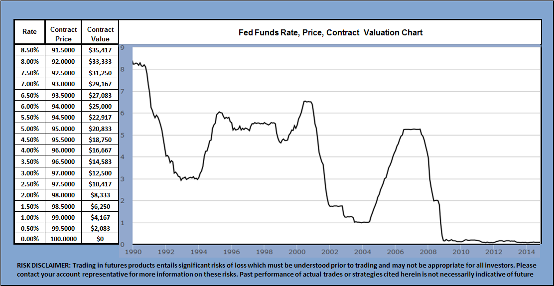
Below is is 1992-2015 rate, price, contract valuation chart Rate is in vertical column 1, contract price 2, contract value 3. Each 0.01 move in this rate equals a $25 change in the contract’s value. Example, a rate of 0.20% = a contract value of $500, at 0.40% the contract value would increase to $1,000 Click here for charts, quotes and historical data from the Federal Reserve Click here to enlarge the chart below
To capture the move you need to trade the underlying futures contract
To convert the contract price into the rate it represents Take 100.0000 – the contract price = the rate, for example 100.0000 – a contract price of 99.7500 = a rate of 0.25% 100.0000 – a contract price of 99.5000 = a rate of 0.50%
To convert rate into contract value Each 0.0100 change in price = $25, 1 full point 1.0000 = $2,500 for example A rate of 0.25% X $2,500 = $625 A rate of 0.50% X $2,500 = $1,250
Trading this rate higher requires establishing ashort position in the underlying futures contract, as the rate rises the futures contract falls in price to reflect the increase in rate/contract value, for example
99.7500 = a rate of 0.25%, contract value of $625 99.5000 = a rate of 0.50%, contract value of $1,250
Click here to enlarge the 1992-2014 monthly rate, price, valuation chart Click herefor a current chart
History of this rate
Gradually, after World War II, the quantity of U.S. dollars outside the United States increased enormously, as a result of both the Marshall Plan and imports into the U.S., which had become the largest consumer market after World War II.
As a result, enormous sums of U.S. dollars were in the custody of foreign banks outside the United States. Some foreign countries, including the Soviet Union, also had deposits in U.S. dollars in American banks, granted by certificates. Various history myths exist for the first Eurodollar creation, or booking, but most trace back to Communist governments keeping dollar deposits abroad.
In one version, the first booking traces back to Communist China, which, in 1949, managed to move almost all of its U.S. dollars to the Soviet-owned Banque Commerciale pour l’Europe du Nord in Paris before the United States froze the remaining assets during the Korean War.
In another version, the first booking traces back to the Soviet Union during the Cold War period, especially after the invasion of Hungary in 1956, as the Soviet Union feared that its deposits in North American banks would be frozen as a retaliation. It decided to move some of its holdings to the Moscow Narodny Bank, a Soviet-owned bank with a British charter. The British bank would then deposit that money in the US banks. There would be no chance of confiscating that money, because it belonged to the British bank and not directly to the Soviets. On 28 February 1957, the sum of $800,000 was transferred, creating the first eurodollars. Initially dubbed “Eurbank dollars” after the bank’s telex address, they eventually became known as “eurodollars” as such deposits were at first held mostly by European banks and financial institutions. A major role was played by City of London banks, as the Midland Bank, now HSBC, and their offshore holding companies.
In the mid-1950s, Eurodollar trading and its development into a dominant world currency began when the Soviet Union wanted better interest rates on their Eurodollars and convinced an Italian banking cartel to give them more interest than what could have been earned if the dollars were deposited in the U.S. The Italian bankers then had to find customers ready to borrow the Soviet dollars and pay above the U.S. legal interest-rate caps for their use, and were able to do so; thus, Eurodollars began to be used increasingly in global finance.
Eurodollars can have a higher interest rate attached to them because of the fact that they are out of reach from the Federal Reserve. U.S. banks hold an account at the Fed and can, ostensibly, receive unlimited liquidity from the Fed should any trouble arise. These required reserves and Fed backing make U.S. Dollar deposits in U.S. banks inherently less risky, and Eurodollar deposits slightly more risky, which requires a slightly higher interest rate.
By the end of 1970 385,000M eurodollars were booked offshore. These deposits were lent on as US dollar loans to businesses in other countries where interest rates on loans were perhaps much higher in the local currency, and where the businesses were exporting to the USA and being paid in dollars, thereby avoiding foreign exchange risk on their loans.
Several factors led Eurodollars to overtake certificates of deposit (CDs) issued by U.S. banks as the primary private short-term money market instruments by the 1980s, including:
The successive commercial deficits of the United States
The U.S. Federal Reserve’s ceiling on domestic deposits during the high inflation of the 1970s
Eurodollar deposits were a cheaper source of funds because they were free of reserve requirements and deposit insurance assessments
Market size
By December 1985 the Eurocurrency market was estimated by Morgan Guaranty bank to have a net size of 1,668B, of which 75% are likely eurodollars. However, since the markets are not responsible to any government agency its growth is hard to estimate. The Eurodollar market is by a wide margin the largest source of global finance. In 1997, nearly 90% of all international loans were made this way
Futures contracts
The Eurodollar futures contract refers to the financial futures contract based upon these deposits, traded at the Chicago Mercantile Exchange (CME). More specifically, EuroDollar futures contracts are derivatives on the interest rate paid on those deposits. Eurodollars are cash settled futures contract whose price moves in response to the interest rate offered on US Dollar denominated deposits held in European banks. Eurodollar futures are a way for companies and banks to lock in an interest rate today, for money it intends to borrow or lend in the future. Each CME Eurodollar futures contract has a notional or “face value” of $1,000,000, though the leverage used in futures allows one contract to be traded with a margin of about one thousand dollars.
CME Eurodollar futures prices are determined by the market’s forecast of the 3-month USD LIBOR interest rate expected to prevail on the settlement date. A price of 95.00 implies an interest rate of 100.00 – 95.00, or 5%. The settlement price of a contract is defined to be 100.00 minus the official British Bankers’ Association fixing of 3-month LIBOR on the day the contract is settled.
How the Eurodollar futures contract works
For example, if on a particular day an investor buys a single three-month contract at 95.00 (implied settlement LIBOR of 5.00%):
if at the close of business on that day, the contract price has risen to 95.01 (implying a LIBOR decrease to 4.99%), US$25 will be paid into the investor’s margin account; or
if at the close of business on that day, the contract price has fallen to 94.99 (implying a LIBOR increase to 5.01%), US$25 will be deducted from the investor’s margin account.
On the settlement date, the settlement price is determined by the actual LIBOR fixing for that day rather than a market-determined contract price.
Futures Contract History
The Eurodollar futures contract was launched in 1981, as the first cash-settled futures contract. People reportedly camped out the night before the contract’s open, flooding the pit when the CME opened the doors. That trading pit was the largest pit ever, nearly the size of a football field, and quickly became one of the most active on the trading floor, with over 1500 traders and clerks coming to work every day on what was then known as the CME’s upper trading floor. That floor is no longer, with the CME having moved over to the CBOT’s trading floor and 98% of Eurodollar trading now done electronically.
Eurodollar futures contract as synthetic loan
A single Eurodollar future is similar to a forward rate agreement to borrow or lend US$1,000,000 for three months starting on the contract settlement date. Buying the contract is equivalent to lending money, and selling the contract short is equivalent to borrowing money.
Consider an investor who agreed to lend US$1,000,000 on a particular date for three months at 5.00% per annum (months are calculated on a 30/360 basis). Interest received in 3 months’ time would be US$1,000,000 × 5.00% × 90 / 360 = US$12,500.
If the following day, the investor is able to lend money from the same start date at 5.01%, s/he would be able to earn US$1,000,000 × 5.01% × 90 / 360 = US$12,525 of interest. Since the investor only is earning US$12,500 of interest, s/he has lost US$25 as a result of interest rate moves.
On the other hand, if the following day, the investor is able to lend money from the same start date only at 4.99%, s/he would be able to earn only US$1,000,000 × 4.99% × 90 / 360 = US$12,475 of interest. Since the investor is in fact earning US$12,500 of interest, s/he has gained US$25 as a result of interest rate moves.
This demonstrates the similarity. However, the contract is also different from a loan in several important respects:
In an actual loan, the US$25 per basis point is earned or lost at the end of the three-month loan, not up front. That means that the profit or loss per 0.01% change in interest rate as of the start date of the loan (i.e., its present value) is less than US$25. Moreover, the present value change per 0.01% change in interest rate is higher in low interest rate environments and lower in high interest rate environments. This is to say that an actual loan has convexity. A Eurodollar future pays US$25 per 0.01% change in interest rate no matter what the interest rate environment, which means it does not have convexity. This is one reason that Eurodollar futures are not a perfect proxy for expected interest rates. This difference can be adjusted for by reference to the implied volatility of options on Eurodollar futures.
In an actual loan, the lender takes credit risk to a borrower. In Eurodollar futures, the principal of the loan is never disbursed, so the credit risk is only on the margin account balance. Moreover, even that risk is the risk of the clearinghouse, which is considerably lower than even unsecured single-A credit risk.
Other features of Eurodollar futures
40 quarterly expirations and 4 serial expirations are listed in the Eurodollar contract. This means that on 1 January 2011, the exchange will list 40 quarterly expirations (March, June, September, December for 2011 through 2020), the exchange will also list another four serial (monthly) expirations (January, February, April, May 2011). This extends tradeable contracts over ten years, which provides an excellent picture of the shape of the yield curve. The front month contracts are among the most liquid futures contracts in the world, with liquidity decreasing for the further out contracts. Total open interest for all contracts is typically over 10 million.
The CME Eurodollar futures contract is used to hedge interest rate swaps. There is an arbitrage relationship between the interest rate swap market, the forward rate agreement market and the Eurodollar contract. CME Eurodollar futures can be traded by implementing a spread strategy among multiple contracts to take advantage of movements in the forward curve for future pricing of interest rates.
In United States banking, Eurodollars are a popular option for what are known as “sweeps“. Until July 21, 2011, banks were not allowed to pay interest on corporate checking accounts. To accommodate larger businesses, banks may automatically transfer, or sweep, funds from a corporation’s checking account into an overnight investment option to effectively earn interest on those funds. Banks usually allow these funds to be swept either into money market mutual funds, or alternately they may be used for bank funding by transferring to an offshore branch of a bank.


 Source Federal Reserve


 Source Federal Reserve


