What is Contango and Backwardation

Metals Educational Video & Link Home Page

Contango and backwardation are terms used to define the structure of the forward curve. When a market is in contango, the forward price of a futures contract is higher than the spot price. Conversely, when a market is in backwardation, the forward price of the futures contract is lower than the spot price.

Contango

In the chart below, the spot price is lower than the futures price which has generated an upward sloping forward curve. This market is in contango – the futures contracts are trading at a premium to the spot price. Physically delivered futures contracts may be in a contango because of fundamental factors like storage, financing (cost to carry) and insurance costs. The futures prices can change over time as market participants change their views of the future expected spot price; so the forward curve changes and may move from contango to backwardation.

Backwardation

In the chart below, the spot price is higher than future prices and has generated a downward sloping forward, or inverted, curve which is in backwardation. The futures forward curve may become backwardated in physically-delivered contracts because there may be a benefit to owning the physical material, such as keeping a production process running. This is known as the convenience yield, which is an implied return on warehouse inventory. The convenience yield is inversely related to inventory levels. When warehouse stocks are high, the convenience yield is low and when stocks are low, the yield is high.

Convergence

Over time, as the futures contract approaches maturity, the futures price will converge with the spot price, otherwise an arbitrage opportunity would exist.

How and Where Precious Metals are Traded

Metals Educational Video & Link Home Page

How and Where Precious Metals Are Traded

Review the marketplaces where precious metals are traded around the world.

Precious metals have always been used as means of exchange between traders and as a store of wealth, with gold being the metal most commonly used for this purpose. Today there are many ways to invest and trade in gold and other precious metals.

Precious Metals Bars

Investing directly in gold bars is a popular way to access these markets. Bars come in many sizes to suit the needs of the investor. One of the largest markets for gold bars is organized in London. Here the standard size of bar is 400 troy ounces, which is referred to in the market as a large bar. Other bar sizes frequently used around the world include 100 troy ounces, 1 kilogram and 5 tael. The standard size for silver bars in the London market is 1,000 troy ounces. For platinum and palladium, the acceptable size in the London market is between 1 and 6 kilograms.

Taking Ownership

Taking direct ownership of precious metals often involves the use of specialist vaulting and custody arrangements, secure transportation and insurance coverage. In addition to direct investment, the London market has also developed a system of indirect investment.

Precious metals can be bought on an unallocated basis through a bank or intermediary. The bank retains control of the metal whilst the buyer holds the metal on account. Owning metal on an unallocated basis introduces an element of counterparty risk, but provides for a more straight-forward mechanism for completing transactions: trades are completed by the banks moving balances between account.

The London markets for precious metals are organized on a private, over-the-counter basis, without a central exchange coordinating trading. In a number of other locations around the world, exchanges have developed to provide trading facilities in metal. One of the most active of these is the Shanghai Gold Exchange, which provides a centralized spot market for gold and silver bars.

Buying Coins

In addition to bars, investors looking for a direct investment in physical gold and silver can also buy coins. Many countries mint coins from gold and silver, and there are many private markets and agencies that support this form of investment.

Indirect Investment

Another popular way to invest in precious metal is through a mutual fund or an exchange traded fund. This is an indirect form of investment, where investors place their assets into a fund and in turn the fund invests in metal. The fund charges a management fee to cover its costs. With an exchange-traded fund, equity in the fund is traded on a stock exchange, with the most active of these funds being listed in New York and London.

Technology is widely used in the trading arrangements for all these products. A new development that is emerging is the is use of blockchain technology to support the ownership and the efficient transfer of precious metal.

Trading Precious Metals

It is difficult to make an accurate assessment of the amount of precious metal that is traded in these markets, as many trades are in private markets that do not report transaction information.

Data for the London market shows that on average over 19 million ounces of gold and 170 million ounces of silver are transferred every day, with the amount traded likely to be a multiple of this. Volumes on the Shanghai Gold Exchange show an average daily trading volume of over 6 million ounces of gold and 140 million ounces of silver. Trading in the shares of the largest exchange-traded fund for gold can be equated to approximately 1 million ounces of gold per day. It is clear that the amount of precious metal traded on the world’s markets is many times the amount produced from mining and recycling activities.

In the middle part of the twentieth century, the U.S. dollar was convertible into gold at a fixed official fixed rate of $35 per ounce, as part of the Bretton Woods system. This convertibility ended in 1971, and the price of gold became subject to the forces of supply and demand. As a consequence, the need for risk management tools developed. Coinciding with a change in U.S. law that had previously barred private ownership of gold, COMEX launched its Gold futures contract in 1974. The COMEX Silver futures contract had been available since 1933.  Platinum futures were launched on NYMEX in 1956, and Palladium futures launched in 1968. Precious metals futures are also available on a number of other exchanges, most notably in Asia, such as the Shanghai Futures Exchange and the Tokyo Commodity Exchange.

Futures contracts provide a mechanism to manage exposure to the underlying market. In the precious metal markets, the futures contracts offered by COMEX, NYMEX and others are a part of the wider global market for precious metals. They provide transparency and price discovery to the market. Options contracts on precious metal and precious metal futures are also offered by exchanges. Options contracts add to the range of trading and hedging strategies that can be employed by an investor.

Volume (2016) in COMEX Gold futures contracts averages the equivalent of 22 million ounces per day. Each contract is for 100 ounces of gold, and is for delivery at specified time in the future. Each COMEX Silver futures contract is for 5,000 ounces of silver. Its traded volume is equivalent to over 350 million ounces per day on average. The NYMEX Platinum contract is for 50 ounces of platinum, and the NYMEX Palladium contract is for 100 ounces of palladium. Together these two contracts trade in excess of 1.25 million ounces of metal per day.

In conclusion, the world’s precious metals markets consist of a wide range of products to invest in, and tools to assist in managing the risks associated with these investments, and the financial risks of dealing in the physical supply chain.

If you have questions send us a message or schedule an online review .

Regards,
Peter Knight Advisor

—————————————————————-

Privacy Notice

Disclosure


Understanding Supply and Demand: Precious Metals

Metals Educational Video & Link Home Page

Precious Metals Supply and Demand

Understanding the forces and drivers of supply and demand in the physical market is essential for understanding the derivatives markets.

Supply

For all four of the main precious metals, gold, silver, platinum and palladium, new supply comes to the market from mining production and recycling of scrap and obsolete material.

Mining product accounts for between 70-85% of the total new supply, depending on the metal, with recycled material accounting for the remainder. The proportion fluctuates with time, reflecting the changing cost of production, reclamation values and the economic outlook, amongst other factors.

Gold

For gold, supply from these two sources amounts to around 120 million troy ounces per year, equivalent to around 3,700 metric tons. This production has a value in the order of $150 billion, which represents the highest value of production in the precious metals space.

Gold mine production comes from countries throughout the world. Chinese mine production has risen considerably in recent years, and now China is the world’s largest producer, accounting for around 16% of global output. In contrast, South Africa, which used to be largest producer has seen declining output in recent years, and now accounts for around 5% of production. Australia, Russia, the U.S., Canada, Mexico, Peru and Ghana also produce significant quantities.

Silver

Silver has the largest supply volume of the four metals at an excess of 30,000 metric tons per annum. This has a value in the order of $17 billion. As with gold, Chinese mine production of silver has increased substantially in recent years, although Mexico remains the largest source of silver mine supply. Australia, Russia and Peru are also significant suppliers of mine production. Silver is often a co-product of the mine production of other minerals, such as gold or copper.

Platinum and Palladium

Platinum and palladium have lower production volumes; 230 metric tons for platinum and 290 metric tons for palladium. South Africa and Russia are the most significant producers of mined metal. For platinum, South African production dominates the market, representing around 2/3 of global mining output.

The mined ore, and recycled metal is refined and normally formed into bars for transportation and storage. Platinum and palladium are also formed into a powder, known as sponge, for use in various industrial applications.

Production from mines and recycling is not the only source of supply to the market. Once manufactured, bars are stored in vaults. The stock of stored metal in these vaults that has accumulated over many years is also available as supply to the market.

There are no reliable estimates of the amount of precious metal stored in vaults. Some is owned by central banks, some is owned by investment funds and some is owned by individual and corporate investors and intermediaries.

Demand

Investment demand is a significant element in the market for precious metals and has an important role to play in establishing market prices for metals. However, investment transactions usually represent the transfer of ownership of stored material. This brings valuable liquidity to the market, but will have little impact on the overall supply and demand. Taken as a whole, investment behavior can be seen as either a net buyer of metal, and therefore a source of demand, or a net seller of metal, and therefore a source of supply. The overall impact of investment will reflect investor sentiment of how ownership of metal will compare to other investment opportunities over their investment horizon.

Gold is the most widely held investment commodity. As well as private investments in gold, central banks hold a significant amount of their reserves in gold. The IMF and the World Gold Council estimate that the world’s central banks hold around 33,000 metric tons of gold, worth over $1 trillion. Changes in this amount will affect the net supply or demand in the market.

Silver is widely used in the production of coins. The U.S. and Canada are the largest producers of silver coins. The U.S. Mint produces in excess of 40 million American eagle silver dollars each year. It is estimated that the global use of silver for coinage accounts for around 14% of annual silver production.

Industrial Use

Also, on the demand side, all four metals have a wide range of industrial uses, reflecting their physical properties.

Gold is used in electronics and in medical and dental applications, amongst other industrial uses.

Silver also has extensive demand from the electronics sector, and has seen increased use in photovoltaic cells. Silver used to be used extensively in photographic production, but this has decreased sharply with the advent of digital photography.

A major use of platinum and palladium is in the creation of vehicle emission control devices. They also have applications in the electronics sector.

Jewelry

Precious metals are also widely used in the manufacture of jewelry. Jewelry use is the primary physical use of gold, with the amount used equating to over 2/3 of annual production, i.e. over 2,500 metric tons each year. The use of silver and platinum for jewelry is relatively lower, at just under 1/3 of annual production. Palladium is used in jewelry, but the amount is much less significant.

Conclusion

In conclusion, thousands of tons of precious metal are produced each year from mining operations, adding to the stock of metal available. These metals are used in industry and in jewelry, from where they can be recycled back into the market.  Precious metal is also held in store as an investment and as part of countries’ official reserves. The combination of all these factors creates an active global market for precious metal.

Further Reading:

1) CPM Group precious metals yearbooks
2) Thomson Reuters GFMS
3) World Gold Council
4) The Silver Institute
5) International Monetary Fund
6) US Geological Survey

If you have questions send us a message or schedule an online review .

Regards,
Peter Knight Advisor

—————————————————————-


Privacy Notice

Disclosure


Defining risk on every trade and for the duration of every trading period 

Defining risk using “option collars

1) Procedure for a Collared Long Position

1.1) On the 15th of September 2017 was telling us the S&P is in a medium-term up trend and to structure trades for 11 to 29 days.

Enter a long futures position at 2,500.00
Contract value $125,000.00

1.2) Determine the profit objective

In this example I’m simplifying the profit objective procedure by extending the angle of the slope using the medium-term EMA9 chart  by the maximum trade duration of 29 days to generate a profit objective of 2,550.00 contract value $127,500.00.

Profit Objective 2,550.00
Contract value $127,500.00

2) Collaring the trade

2.1) At the 2,550.00 profit objective I sell an out of the moneycall option against the my long position at the closest strike price to the objective of 2,550,00.

2.2) I’ll chose an options expiration that is consistent with the maximum trade duration for the trade, in this example 29 days, 13th of October 2017.

2.3) When you sell a call  against your 2,500.00 long futures position (covered call) you’re collecting option time premium, in this example we’ve collected 15.00 points or +$750.00.

How we objectively define risk

2.4) Using the collected premium from the covered call of 15.00 points, ($750.00)  I buy a put option.

2.4) The put option purchased must have the same option expiration as the call we wrote, in this example the option expiration for the call we wrote is the 13th of October 2017, the put purchased must have the same expiration date.

2.5) The put  strike price should be approximately the same distance from our 2,500.00 long entry as the call we wrote at the 2,550 objective (50 points).
2,500.00 entry – 50.00 = 2,4550.00, the put I purchase to define my risk should be at a strike of 2,450.00 or higher.

2.6) The option premium price paid for the put option to define risk should be approximately the same amount as what I’ve collected from the call I wrote. (In this example I’ve collected 15.00 points ($750.00) on the call, the put protection premium should cost me approximately 15.00 points  ($750.00).

2.7) Purchase the 2,450.00 put with the same expiration date for 17.00 points ($850.00).

2.8) The put objectively defines my risk on the 2,500.00 long position for the duration of the trading period (entry date 15 September 2017 to 13 October 2017 expiration)

2.9) The put also negates any possibility of this position being stopped out for the duration of the trading period.

2.10) Summary
Long a futures contract at 2,500.00
Collected on the 2,550.00 call write, 15.00 points at the profit objective
Paid out on the 2,450.00 put purchase -17.00 points to objectively define risk

Net cost of the hedge = 2.00 points or $100.00,  which defines risk on a contract worth $125,000 from the 14th of September 2015 until  the 13th of October 2017. 

3) Potential outcomes

3.1) The market stays the same and settles on the 13th of October 2017 at 2,500.00 unchanged from entry.

3.2) Trade Result

The call we wrote at 2,550 expires worthless, +15.00 points = +$750.00

The 2,500.00 long futures settles unchanged at 2,500.00 = $0.00

The 2,450 put purchased expires worthless, we lose 17.00 points = -$850.00

Total bid/ask spreads, commission, exchange & regulatory fees =-$159.78

All in net profit or loss = -$259.78

3.3) The market moves hard against us

The market drops from our entry price of 2,500.00 (contract value = $125,00.00) down 600.00 points -24.00% to 1,900.00 contract value $95,000 in fast market action.

If a percentage drop like this occurred, it would have no impact on the maximum risk of this collared position because we own the put.

The maximum risk (in this example) is the distance between our entry at 2,500.00 contract value $125,000.00 to where the put engages at 2,450.00, contract value $122,250.00, maximum loss $2,500.00 regardless if this market moves to zero.

3.4) Trade Result

Loss on the 2,500.00 long futures position (600.00) points = -$30,000.00

The call we wrote at 2,550.00 expires worthless +15.00 points =+$750.00

The put we own at 2,450.00 is profitable 533.00 points =+$26,650.00

Total bid/ask spreads, commission, exchange & regulatory fees =-$159.78

All in net loss = -$2,759.78

A $100.00 hedge prevented a potential loss on this position of $30,000.

3.5) The market moves higher in our favor 

The established trend continues higher  from our long entry of 2,500.00 contract value $125,000 to our profit objective of 2,550.00 contract value $127,500 on or before the 13th of October 2017.

3.6) Trade Result

Gain on the 2,500.00 long futures position 50.00 points = +$2,500.00

The covered call we wrote at 2,550.00 is offset by the futures, we also keep the 15.00 points in collected premium =+$750.00

The put we own at 2,450.00 expires worthless -17.00 points =-$850.00

Total bid/ask spreads, commission, exchange & regulatory fees =-$159.78

All in net profit or loss = $2,240.22.

4) Procedure for short positions
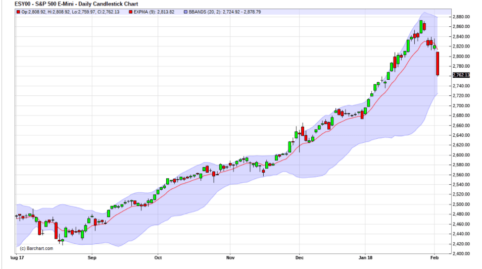
4.1) On the 1st of  February 2018 (TIPTrend identification procedure linked here  is telling you the S&P is in a short-term downtrend and to structure a short trade for 2 to 10 days.

We enter a short futures position at 2,815.00
Contract value $140,750.00

4.2) Determine the profit objective

To simplify I am continuing the angle of the slope on the short-term EMA9 chart out 10 days to generate a profit objective of 2,740.00

Profit objective at 2,740.00
Contract value $137,500.00

5) Collar procedure

Short futures on 2 February 2018 at 2,815 (contract $140,750.00)

5.1) I write an out of the money, put option against my 2,815.00 short futures position at the strike price that is closest to the profit objective, in this example 2,740.00

5.2) I choose an options expiration that is consistent with the TIP  defined trade duration (in this example the 9th of February 2018).

5.3) When I write an out of the money option against my short position I collect option premium, in this example I’ve collected 27.00 points or +$1,350.00.

Objectively Defining Risk

5.4) Using the collected premium of 27.00 points or +$1,350.00 from the sale of the 2,740.00 put I buy a call option.

5.5) The call option purchased must have the same option expiration as the put I wrote (in this example the 9th of February 2018).

5.6) The option premium price paid for the call option should be approximately the same amount or less than what I’ve collected from the put write (in this example I collected 27.00 points or +$1,350.00).

5.7) The call strike price should be approximately the same amount from entry. In this example I’m short futures at 2,815.00 , I written an out of the money put at my profit objective 75.00 points below my 2,815 short entry , the call I purchase should be at a strike of 2,815.00 + 75.00 = 2,890.00 or lower.

5.8) I purchase the 2,890.00 call with an expiration date of the 9th of February 2018 for 16.00 points  or –$800.00.  

5.9) The call objectively defines risk on my 2,815.00 short position for the duration of the trading period (entry date 2nd of February 2018 to the 9th of February 2018 expiration)

5.10) The call negates any possibility of this position being stopped out for the duration of the trading period.

5.11) Summary

Short a futures contact at 2,815.00
On the put write at my profit objective of 2,740.00 I’ve collected 27.00
I’ve paid out 16.00 points on the 2,890.00 call to objectively define my risk

Net cost of the hedge = +9.00 points or $550.00,  in this example we I’m getting  paid to define risk on a contract worth $140,750 from the 2nd of February 2018 to the 9th of February 2018 . 

6) Potential outcomes for this trade

6.1) The market stays the same and settles on the 9th of February 2018  unchanged from our entry at 2,815.00.

6.2) Trade Result

The put wrote at 2,740.00 expires worthless, I keep the 27.00 points = $1,350.00

The 2,815.00 short futures settles unchanged at 2,815.00 = $0.00

The 2,890.00 call purchased expires worthless, I lose 16.00 points = -$800.00

Total bid/ask spreads, commission, exchange & regulatory fees = -$159.78

All in net profit or loss  = +$390.22

6.3) The market moves hard against us

The market rallies from my short entry at 2,815.00 (contract value = $144,500.00)  300.00 points +10.66% to 3,115.00 contract value $155,750 in “fast market action.

If a  rally like this occurred it would have no impact on the maximum risk of this collared position because I own the call.

The call objectively defines my risk on the this short position for the duration of the trading period. The maximum risk (in this example) is the distance between my entry at 2,815.00 contract value $140,750.00 to where the call engages at 2,890.00 contract value $144,500.00

6.4) Trade Result

Loss on the 2,815.00 short futures position 300.00 points = -$15,000.00

The put I wrote at 2,7400 expires worthless +27.00 points =+$1,350.00

The call I own at 2,890.00 is profitable by 209.00 points =+$10,450.00

Total bid/ask spreads, commission, exchange & regulatory fees = -$159.78

Net loss = -$3,359.78.78

In this example I was paid $+550.00 to prevent a potential loss of $15,000

6.5) Market moves lower in my favor

The trend continues lower from my short entry at 2,815.00 on the 1st of February 2018 contract value $140,750.00 to my profit objective of 2,740.00 contract value $137,000 on or before the 9th of February 2017.

6.6) Trade Result

Gain on the 2,815.00 short futures position 75.00 points = $3,750.00

The put I wrote at 2,740.00 is offset by the short futures position, I keep the +27.00 points in collected option time premium = +$1,350.00

The call I purchased at 2,890.00 expires worthless -18.00 points = -$800.00

Total bid/ask spreads, commission, exchange & regulatory fees = -$159.78

All in net gain or loss = $4,140.22

7) S&P Collar Spreadsheet

  • Open with Excel
  • Click OK
  • Enable editing
  • Enable content

If you have questions or need help with this procedure please schedule an online review or send me a message

Regards,
Peter Knight Advisor
Contact

____________________________________________________________________________

Privacy Notice

Disclosure


Defining Trend, Reversals, Trade Duration & Number of Contracts Traded

This program trades up to 5 S&P E-mini contracts per $25,000 trading unit with the trend up or down using defined risk strategy. The Gold ATA and Currency ATA’s use the same methodology.

  • Up toshort-term positions with a trade duration of 2 to 10 days
  • Up tomedium-term positions with a trade duration of 11-29 days
  • Up to long-term position, trade with a duration of 30 to 90 days
  • Total margin requirement never exceeds $12,500 USD per $25,000 USD  trading unit because all trades are fully hedged.

1) Trend Identification Procedure (TIP)

1.1) Looking at the 1983 to 2018 chart below and linked here does it really look that hard to identify the major up or downtrends over the last 35 years?

1.2) One quick and reliable indicator out of the 12 this program uses is an Exponential Moving Average 9 (EMA9).

On the 2000 to 2013 chart below and linked here I’ve dropped in an EMA9 represented by the red line.

1.2) Whatever data period you’re using, 3 minutes to 3 months if price action is below the (EMA9) it’s telling you the market is in a downtrend.

1.3) If price action is above the (EMA9) an uptrend

1.4) By itself you’ll find the EMA9 a quick and reliable way to initially qualify a market’s trend.

Below I’ve linked every Bull and Bear market since 1983 enabling you to review the accuracy of the EMA9 as an indicator. These charts should also clarify the need to trade the market both long or short to maximize profitability.

1.5)  1983-2018 chart 
1.6) January 1983 – August 1987  Bull 139.72 – 337.89 =+141.83%
1.7) August 1987 – October 1987 Bear 337.89 – 216.47 =-35.94%
1.8) August 1987 – August 1989  Bear to recovery (2 years)

1.9) August 1987 – July 1990  Bull 216.47 – 369.78 = +70.82%
1.10) July 1990  October 1990  Correction  369.78 – 294.51 =-20.36%
1.11) July 1990 – February 1991  Correction to recovery (7 months)

1.12) October 1990 – July 1998  Bull 294.51 – 1,190.58 =+304.26%
1.13) July 1998 – October 1998 Correction 1,190.58 – 923.52 =-22.43%
1.14) July 1998 – November 1998  Correction to recovery (4 months)

1.15) October 1998 – March 2000 Bull 923.52 – 1,552.87 =+68.15%
1.16) March 2000 October 2002  Bear 1,52.87 – 768.63 =-50.50%.
1.17) March 2000 December 2007 Bear to recovery (7 years 9 months)

1.18) October 2002 – October 2007   Bull 768.63 – 1,576.09 =+105.05%
1.19) October 2007 –  March 2009  Bear 1,576.09 – 666.79 =-57.70%
1.20) October 2007-  April 2013  Bear to recovery (5 years 6 months)

1.21) March 2009 – January 2018  Bull 666.79 – 2,872.87 = +327.87%

2) Once you’ve initially qualified the trend using the EMA9 confirm the trend using the overall average of the indicators linked here.

3) Specific examples 

3.1) Short-term trades with a trade duration of 2 to 10 days

In the example below is the daily price action above or below the EMA9?

Above the EMA9 = buy
Below the EMA9 = sell

Below, the short term trend is down

3.3) Confirm the EMA9 short-term trend using the overall average and the short-term technical opinion.

In this example the overall average is a 48% sell
The average of the 5 short-term indicators is a 60% sell

3.4) If the EMA9, overall average and short-term average indicators all agree short-term trades of 2 to 10 days in duration are permitted

Example,

EMA9 = sell
Overall average = 48% sell
5 short-term indicators = 60% sell

If you’re already short the market, short-term trades can be maintained, if you’re long reverse to short.

This program trades up to 2 short-term positions per $25,000 trading unit.

3.5) Short-term, short futures positions with a duration of  2 to 10 days 

If the overall average and short-term average indicators are less than a 50%  sell you are not permitted to add a second position

Example,

Overall average =  65% sell
5 short-term indicators =  40% sell
Does not permit adding a second contract 

If the overall average and short-term average indicators are both greater than a 50% sell you are permitted to add a second position

Example,

Overall average = 53% sell

5 short-term indicators = 60% sell
Permits a second contract  

3.6) Short-term, long futures positions with a duration of  2 to 10 days 

If the overall average of short-term average indicators are less than a 50%  buy you are not permitted to add a second position

Example,

Overall average = 60% buy
5 short-term indicators = 35% buy
Does not permit a second contract

If both the overall average and short-term average indicators are greater than a 50% buy you are permitted to add a second position

Example,

Overall average = 53% buy
5 short-term indicators = greater than  60% buy
Permits a second contract

3.7) If the EMA9, overall-average and short-term average indicators do not  agree liquidate to neutral.

Example,

EMA9 using daily data = buy (price action is above the EMA9)
Overall average = 27% Buy 
5 short-term indicators = 8% sell
Liquidate

Try to identify today’s short-term trend 

3.6) Today’s EMA9 (using daily data)

  • Is price action above or below the EMA9?
  • Above = BUY
  • Below = Sell

3.7) Today’s Technical (Opinion)

  • Does the overall average agree with the EMA9?
  • Does the average of the 5 short-term indicators agree with the EMA9?
  • If they all agree positions are permitted
  • If the overall average and short-term indicators are greater than 50% a second position is permitted
  •  If they disagree liquidate to neutral

3.8) Once trend is defined “collar” the trade, using this procedure.

  • Collars objectively define risk on the trade and for the duration of the trading period
  • Collars eliminate any possibility of the position being stopped out
  • Collars eliminate the possibility of a margin call (because risk is objectively defined when the trade is established)
  • In most cases collars reduce your margin requirement, if the maximum risk on the trade is $1,800.00 and the exchange margin requirement is $5,050.00, the margin requirement would be the lower of the 2, in this example the margin requirement would be the maximum trade risk of $1,800.00.
  • Properly set up a collar is premium neutral (does not waste investment capital on excessive purchases of option time premium to define risk)

4) Medium-term trades with a duration of 11 to 29 days

4.1) The rules are the same as the short-term but you’re using an EMA9 on weekly price action versus daily

4.2) Confirm the EMA9 medium-term trend using the overall average  and medium-term average of technical opinions.

In this example the overall average is a 48% sell
The average of the 5 short-term is a 50% sell

Try to identify today’s medium-term trend

4.3) Today’s EMA9  (using weekly data) 

  • Is price action above or below the EMA9?
  • Above = BUY
  • Below = Sell

4.4) Today’s indicators (Opinion)

  • Does the overall average agree with the EMA9?
  • Does the average of the 4 medium-term indicators agree with the EMA9?
  • If they all agree positions are permitted
  • If the overall average and medium-term indicators are greater than 50% a second position is permitted
  •  If they disagree liquidate to neutral

4.5) Once a trend is defined “collar” the trade, using this procedure.

5) Long-term trades with a duration of 30 to 90 days

5.1) The rules are the same as the short-term but you’re using an EMA9 on monthly price action versus daily or weekly.

5.2) Confirm the EMA9 long-term trend using the overall  average and long-term Average technical opinions.

In the example below, the overall average was a 48% sell, the long-term indicators are generating a hold, no new long-term trades would  be permitted.

5.3) This program trades a maximum of 1 long-term position per $25,000 trading unit.

Try to identify today’s long-term trend

5.4) Today’s EMA9  (using monthly data)

  • Is price action above or below the EMA9?
  • Above = BUY
  • Below = Sell

5.5) Today’s indicators (Opinion)

  • Does the overall average agree with the EMA9?
  • Does the average of the 3 long-term indicators agree with the EMA9?
  • If they all agree positions are permitted
  •  If they disagree liquidate to neutral

5.6) Once trend is defined collar the trade, using this procedure.

6) To demonstrate the durability of the EMA9 and Opinion try using them on the related and unrelated markets linked below.

6.1) Last 10 EuroStoxx  
6.2) Opinion
6.3) Last 10 FTSE 100 monthly O/H/L/C
6.4) FTSE opinion
6.5) Last 10 DAX Index monthly O/H/L/C
6.6) DAX Index opinion
6.7) Last 10 Gold monthly O/H/L/C
6.8) Gold opinion
6.9) Last 10 Euro monthly O/H/L/C
6.10) Euro opinion
6.11) Last 10 British Pound monthly O/H/L/C
6.12) British Pound opinion
6.13) Last 10 Australian dollar monthly O/H/L/C
6.14) Australian Dollar opinion
6.15) Last 10 Canadian dollar monthly O/H/L/C
6.16) Canadian Dollar opinion
6.17) Last 10 Brazilian Real monthly O/H/L/C
6.18) Brazilian Real opinion
6.19) Last 10 Russian Ruble monthly O/H/L/C
6.20) Russian Ruble opinion
6.21) Last 10 on 2 year US Treasuries monthly O/H/L/C
6.22) 10 Year Treasury opinion
6.23) Last 10 Euro Bund  monthly O/H/L/C
6.24) Euro Bund opinion
6.25) Last 10 NY Crude Oil monthly O/H/L/C
6.26) Crude Oil opinion
6.27) Last 10 Copper monthly O/H/L/C
6.28) Copper opinion
6.39) Last 10 Lumber monthly O/H/L/C
6.30) Lumber opinion
6.31) Last 10 Cotton monthly O/H/L/C
6.32) Cotton opinion
6.33) Last 10 Orange Juice monthly O/H/L/C
6.34) Orange Juice opinion

Identifying the trend is only 1/3rd of the battle to win the war of becoming a profitable trader, the other 2/3rds is how you structure your trades.

For full disclosure of how we set profit objectives and define risk on every trade and for the duration of every trading period see this link.

If you have questions send us a message or schedule an online review .

Regards,
Peter Knight Advisor

—————————————————————-

Privacy Notice

Disclosure


About S&P Futures Contracts

Stock Index Education Home Page

If you’re not familiar with futures contracts they are agreements to buy or sell at an agreed price on or before an agreed date.

Long = own the contract anticipating the price to move higher, once a long position is established it has to be sold on or before the contract delivery date, for example an ESH18  contract has to be offset or before March 16th 2018.

Short = Owe the contract, selling a contract you do not own, once a short position is established it has to be bought back on or before the delivery date, Trading futures there is no dividend delivery, no short squeezes.

Contract value = $50 X the index, (an index at 2,825.00 = $141,250.00)
Bid/ask spread 0.25 = $12.50 , contract value = $141,250.00 at 2,825.00
Margin requirement = $5,050.00 (1/28th of contract value)
Margin call, if your balance falls below the margin requirement
Carry cost built into forward pricing  (current leverage cost 0.73% annually)
Trade cost, $26.60 or less per contract (includes all fees)
Contract volume, 130+ billion USD daily, liquid underlying options market

One click lets you go long or short a contract that mirrors the S&P index (worth $141,250.00 at 2,825.00) with as little as $5,050 in your account.

Long short flexibility

A 23.75 hour trading day and 130+ billion USD in daily liquidity make it very easy on days like 2nd and the 5th of February 2018 to hedge an existing portfolio or capture the move lower.

Contract value is based on these 500 stocks

Quotes, charts and analysis for all 500 stocks
SEC filings & information for all 500 stocks

Trading Hours
CME Globex: Sunday – Friday 6:00 p.m. – 5:00 p.m. Eastern Time (ET) with  trading halt 4:15 p.m. – 4:30 p.m. Clearport: Sunday – Friday 6:00 p.m. – 5:00 p.m. ET

Margin Requirement

Product Code
CME Globex: ES

CME ClearPort: ES
Clearing: ES

Listed Contracts
Four months in the March Quarterly Cycle (Mar, Jun, Sep, Dec)

Termination Of Trading
9:30 a.m. ET on the 3rd Friday of the contract month

Position Limits (excel file)  

Exchange Rulebook

If you have questions send us a message or schedule an online review .

Regards,
Peter Knight Advisor

—————————————————————-

Privacy Notice

Disclosure

Equity Index Daily & Final Settlement

Stock Index Education Home Page

Equity Index Daily & Final Settlement

When trading Equity Index futures, there are two types of settlement: daily and final.

Daily settlement refers to the contract’s settlement price on a daily basis while final settlement represents the final value of the contract at expiration

Futures markets are marked to market every day, a benefit that means every market participant sees the same settlement price at the same time as every other participant.

Daily Settlement

For most Equity Index futures, daily settlement price for the front month is calculated using a volume weighted average price (VWAP) based on the last 30 seconds of the trading day.

In the case of the E-Mini NASDAQ-100 futures contract, the average would be based on trading activity on CME Globex between 15:14:30 – 15:15:00 Central Time.

Traders, brokers, and others market participants use daily settlement information to manage daily profit and loss, as well as to possibly adjust their margin levels with their clearing firms.

Final Settlement

When it comes to final settlement for U.S.-based Equity Index contracts, the value is determined using a Special Opening Quotation, known as the SOQ.

The SOQ is determined by the index provider and is calculated using the actual opening prices for each of the underlying constituent stocks.

In the case of S&P500® futures, the SOQ is determined by the first traded price for each of the 500 companies’ shares that make up the index.

This number is calculated by the Standard and Poors Corporation and generally made available the third Friday of every quarterly futures contract month.

If you have questions send us a message or schedule an online review .

Regards,
Peter Knight Advisor

—————————————————————-

Privacy Notice

Disclosure


Understanding Implied Liquidity in Select Sector Futures

Stock Index Education Home Page

Understanding Implied Liquidity in Select Sector Futures

Liquidity for equity index futures is often measured by what investors can see quoted or traded on-screen. If the central limit order book (CLOB) displays a wide bid-ask spread or shows small size, you may incorrectly conclude that the contract is illiquid. However, with the multitude of ways to trade futures, such as through the CLOB, Basis Trade at Index Close, Block Trades or Exchange for Physicals, you can tap into additional sources of liquidity.

Finding Additional Sources of Liquidity

Consider, a fund manager that needs to trade $25 million in the Financial Select Sector Index intraday, and prefers to trade capital efficient futures. The manager calculates a need to buy 425 XAF contracts to achieve the desired exposure. The manager sees a three-tick wide market on 15 contracts and notices that XAF trades ~300 contracts per day on average. While realizing that working the order may take too long and may result in price slippage, the manager contacts his/her broker or a futures’ block liquidity provider, and indicates interest in a block trade.

BLOCK TRADE

A futures block trade allows participants the flexibility to privately negotiate larger transactions at fair and reasonable prices. The dealer will most likely provide a market based on the liquidity of the underlying single-stock index constituents or the corresponding ETF. By taking advantage of the activity in adjacent markets, the block provider may quote prices on quantities, more than what could be seen on the futures CLOB. In this case, for a $25 million Financial Select Sector futures block trade, the dealer could easily combine its hedge from the nearly $30 billion that trades daily in the underlying stocks and the corresponding ETF market.

BASIS TRADE AT INDEX CLOSE (BTIC)

When participants seek intraday liquidity via blocks, the tightness and size of markets can be affected by the dealer’s ability to hedge the associated risk in the continuous cash market. One way to access additional liquidity for size is to align the futures block execution against the close, to leverage the volume transacted in the index component market-on-close (MOC) auctions. The best way to achieve this alignment is to utilize BTIC block trades. A BTIC block trade enables investors to trade futures at a negotiated spread to the underlying cash index official close and thus provides participants price and size certainty.

To execute a BTIC block, a fund manager needs to reach out to a liquidity provider and negotiate the fair value spread, or basis, of the futures to the Index, say -1.50 index points. The dealer may hedge the BTIC futures trade by buying the required number of shares per component in each stock’s respective MOC auction and perfectly replicating the cash index closing value. If the official index close was 241.5, the 425 futures contracts would be executed at 240.00 via the BTIC block. This enables a fund manager to execute a full order in one trade with price certainty, and encourages a dealer to trade more size via BTIC as a result of the hedge certainty provided by transacting stock in the MOC auction.

EXCHANGE FOR PHYSICAL (EFP)

A third way to access futures exposure is by tapping into the liquidity of the ETF market and then converting the ETF position into futures via an Exchange For Physical (EFP) transaction. EFP transactions are also privately negotiated.

For example, a fund manager purchased ~1 million shares of the Financial Select Sector ETF at a price of $25 to use liquidity in the ETF market, the fund manager could then negotiate an EFP with a dealer to exchange the ETFs for an equivalent futures position using E-mini Financial Select Sector Futures contracts.

Summary

The complete liquidity profile for a futures contract is dependent on the availability of equivalent and substitute products that market makers can use to price and hedge the futures, as well as the availability of exchange mechanisms such as blocks, BTIC and EFPs that can be used to access the contracts. CME Group offers exposure to benchmark equity indices where both on- and off-screen liquidity can be accessed to best meet your risk management needs.

If you have questions send us a message or schedule an online review .

Regards,
Peter Knight Advisor

—————————————————————-

Privacy Notice

Disclosure

How to Trade Select Sectors

Stock Index Education Home Page

Understanding Equity Index Select Sectors

Investors understand that the economy is comprised of various sectors. Of course, some sectors will outperform others at times. Because of this, investors may wish to trade in certain sectors at a given time and other sectors at other times. This decision will be based on your understanding of current market conditions and trends. Like all investment decisions, it should be based on sound research.

How We Can Help

We trade E-mini S&P Select Sector futures contracts, which have multiple applications. They can be used individually to adjust a portfolio’s sector weightings, spread against each other as a relative value trade or simply traded outright, expressing a tactical market view.

Benefits

E-mini Select Sector futures at CME Group offer you the ability to access the individual S&P Select Sectors around-the- clock via CME Globex. All 500 S&P Index stocks are categorized into a specific sector. Flexible execution methods are available – Central limit order book via CME Globex, Block Trades, Basis Trade at Index Close (BTIC) Block Trades, and Exchange for Physical (EFP) trades.

Further benefits include:

Low cost, low tracking error, zero management fees and SOQ settlement at expiration

Spreading opportunities – sector index versus components, sector versus sector and sector versus broad-based

E-mini S&P Select Sector Futures

For risk managers and investors seeking a more refined and targeted sub-sector tool CME Group offers ten flexible E-mini S&P Select Sector futures contracts:

Technology
Health Care
Utilities
Consumer Staples
Financial
Consumer Discretionary
Energy
Materials
Industrial
Real Estate

Designed to closely match the performance of each sector within the S&P 500, E-mini S&P Select Sector futures can be used individually to adjust sector weights, as in a sector rotation strategy. What’s more, these futures contracts deliver several potential margin efficiencies with other equity index futures, a benefit that may not be available by simply holding an underlying basket of stocks or ETFs. Because each constituent of the S&P 500 index is categorized into a specific sector, portfolio managers and investors with changing risk evaluation levels can use E-mini S&P Select Sector futures to manage the desired level of sector risk of their equity portfolio objectives, as illustrated below. Be aware that asset managers routinely trade and rebalance between specific sectors. Additionally, over-weight and under-weight sector strategies are employed to capture alpha, or for market timing.

EXAMPLE

Let’s say that a portfolio manager has a $100,000,000 fund indexed to the S&P 500. Looking forward, he decides to rotate the portfolio, increasing exposure to utilities and also decreasing exposure to financials by 5%.

The portfolio manager elects to adjust his $100 million portfolio using Select Sector futures. He will buy Utilities Select Sector Futures and sell Financial Select Sector futures, as shown below.

$100,000,000 x 5% = $5,000,0000

Hedge Ratio (HR) = Value at risk ÷ Notional Value (NV) Sector futures

HR Utilities = 5,000,000 ÷ (430.00 x 100) = Buy 116 IXSM6 contracts

HR Financials = 5,000,000 ÷ (232.35 x 250) = Sell 86 IXAM6 contracts

In buying 116 contracts of utilities and selling 86 contracts of financials, he has effectively rotated his portfolio away from financials and toward utilities without changing the physical portfolio.

Summary

Sector rotation is a commonly employed financial strategy. It allows traders to lessen risk by increasing exposure to one sector while minimizing exposure to other sectors. E- mini Select Sector futures at CME Group offer the ability to access the individual S&P Select Sectors around-the- clock via CME Globex. In addition to providing capital efficiency, flexible execution methods are available.

If you have questions send us a message or schedule an online review .

Regards,
Peter Knight Advisor

—————————————————————-

Privacy Notice

Disclosure


Equity Intermarket Spreads

Stock Index Education Home Page

 Understanding Intermarket Spreads

A trader can spread between two highly correlated futures contracts of similar but different types. This is known as an inter-market spread.

In the financial futures markets, inter-market spreads can involve trading in highly correlated contracts of different types. For example, you could take a spread position between two different stock indexes by buying one and selling another. If you’re bullish on the technology sector versus the broad market, you could buy the NASDAQ futures and sell the E-mini S&P.

The point of entering into an inter-market spread is to trade on the differences in the two respective contracts rather than the direction of the overall market. These types of trades are sometimes referred to as relative value trades.

Risks and Opportunities

Spread trading does involve risk, and in fact you can lose money on both sides (positions) of the spread. However, spread trading offers unique opportunities that differ considerably from outright long or short positions.

In order to utilize perceived spread opportunities, traders must know the economic fundamentals of the market; this includes a seasonal and historic knowledge of price patterns. Traders must be able to recognize the potential for widening or narrowing changes between contracts and to make that spread change work in their favor.

If you have questions send us a message or schedule an online review .

Regards,
Peter Knight Advisor

—————————————————————-

Privacy Notice

Disclosure