This Spreadsheetwill enable you to create your own allocations providing;
1) Cell B-2 Cumulative net profit, trading with strategies of your choice
2) Cell B-3 Average annual profit
3) Cell B-4 Average monthly profit
4) Cells B-9 through B-33 cumulative net profit/loss per year.
5) Cells C-31 through C-6438 monthly net profit/loss.
6) Cells E-9 through E-6438 cumulative daily market-to-market allocation performance.
7) Horizontal line 7 links to all supporting historical data, orders and trades generated including full disclosure for that trading methodology enabling performance verification.
8) Horizontal line 8 net performance trading 1 mini contact from 1992-2016 for that strategy.
9)Horizontal lines 9 through 6,425 mark-to-market daily performance for that strategy.
Creating your own allocation
Let’s assume you wanted to eliminate any strategy that made less than $65,000 for the life of the program.
Strategies you’d be eliminating CHF006R, CHF007R, EUR002R, EUR003R, EUR004R, EUR006R, JPY006T, JPY009T and JPY019T.
To delete these strategies from your allocation, right click on the vertical columns containing the strategies, left click and delete, repeat until all desired strategies are deleted.
The spreadsheet summaries will reflect the changes.
Adding strategies to trade multiple contracts
Let’s assume you wanted to add CHF positions, left click to highlight the system(s) you’d like to trade multiple contracts of, right click and copy.
Left click and insert cells.
Summaries will automatically update.
If you have any questions or need help using this spreadsheet contact me
PROGRAM AVAILABILITY IS DEPENDENT ON YOUR COUNTRY OF RESIDENCY AND FINANCIAL STATUS
PAST PERFORMANCE IS NOT NECESSARILY INDICATIVE OF FUTURE PERFORMANCE. THE RISK OF LOSS IN TRADING FOREX OR FUTURES CONTRACTS OR OPTIONS CAN BE SUBSTANTIAL, AND THEREFORE INVESTORS SHOULD UNDERSTAND THE RISKS INVOLVED IN TAKING LEVERAGED POSITIONS AND MUST ASSUME RESPONSIBILITY FOR THE RISKS ASSOCIATED WITH SUCH INVESTMENTS AND FOR THEIR RESULTS.
BID/ASK SPREADS, BROKERAGE COMMISSION, CLEARING, EXCHANGE AND REGULATORY FEES WILL HAVE AN ADVERSE IMPACT ON THE NET OVERALL PERFORMANCE OF YOUR ACCOUNT. PRIOR TO MAKING A DECISION TO PARTICIPATE IN ANY INVESTMENT MAKE SURE YOU FULLY UNDERSTAND THE FEES ASSOCIATED WITH TRADING.
EXAMPLES OF HISTORIC PRICE MOVES OR EXTREME MARKET CONDITIONS ARE NOT MEANT TO IMPLY THAT SUCH MOVES OR CONDITIONS ARE COMMON OCCURRENCES OR ARE LIKELY TO OCCUR.
HYPOTHETICAL PERFORMANCE RESULTS HAVE MANY INHERENT LIMITATIONS, SOME OF WHICH ARE DESCRIBED BELOW. NO REPRESENTATION IS BEING MADE THAT ANY ACCOUNT WILL OR IS LIKELY TO ACHIEVE PROFITS OR LOSSES SIMILAR TO THOSE SHOWN IN FACT, THERE ARE FREQUENTLY SHARP DIFFERENCES BETWEEN HYPOTHETICAL PERFORMANCE RESULTS AND THE ACTUAL RESULTS SUBSEQUENTLY ACHIEVED BY ANY PARTICULAR TRADING PROGRAM. ONE OF THE LIMITATIONS OF HYPOTHETICAL PERFORMANCE RESULTS IS THAT THEY ARE GENERALLY PREPARED WITH THE BENEFIT OF HINDSIGHT.
IN ADDITION, HYPOTHETICAL TRADING DOES NOT INVOLVE FINANCIAL RISK, AND NO HYPOTHETICAL TRADING RECORD CAN COMPLETELY ACCOUNT FOR THE IMPACT OF FINANCIAL RISK IN ACTUAL TRADING. FOR EXAMPLE, THE ABILITY TO WITHSTAND LOSSES OR TO ADHERE TO A PARTICULAR TRADING PROGRAM IN SPITE OF TRADING LOSSES ARE MATERIAL POINTS WHICH CAN ALSO ADVERSELY AFFECT ACTUAL TRADING RESULTS. THERE ARE NUMEROUS OTHER FACTORS RELATED TO THE MARKETS IN GENERAL OR TO THE IMPLEMENTATION OF ANY SPECIFIC TRADE PROGRAM WHICH CANNOT BE FULLY ACCOUNTED FOR IN THE PREPARATION OF THE HYPOTHETICAL PERFORMANCE RESULTS AND ALL OF WHICH CAN ADVERSELY AFFECT ACTUAL TRADING RESULTS.
YOU SHOULD CAREFULLY CONSIDER WHETHER SUCH TRADING IS SUITABLE FOR YOU IN LIGHT OF YOUR CIRCUMSTANCES AND FINANCIAL RESOURCES.
THE INFORMATION PROVIDED IN THIS REPORT CONTAINS RESEARCH, MARKET COMMENTARY AND TRADE RECOMMENDATIONS. YOU MAY BE SOLICITED FOR AN ACCOUNT BY ONE OF OUR REPRESENTATIVES OR EMPLOYEES. IT SHOULD BE KNOWN THAT THE REPRESENTATIVES OF OUR FIRM MAY TRADE FUTURES AND OPTIONS FOR THEIR OWN ACCOUNTS OR THOSE OF OTHERS. DUE TO VARIOUS FACTORS (SUCH AS MARGIN REQUIREMENTS, RISK FACTORS, TRADING OBJECTIVES, TRADING INSTRUCTIONS, TRADING STRATEGIES, AND OTHER FACTORS) SUCH TRADING MAY RESULT IN THE LIQUIDATION OR INITIATION OF FUTURES OR OPTIONS POSITIONS THAT DIFFER FROM THE OPINIONS AND RECOMMENDATIONS FOUND IN THIS REPORT.
Performance dates 2 January 1992 through 31 August 2016 No compounding of positions, withdrawing all gains annually
Net performance = +$1,817,895
Net profit 2015 = +$115,898
Net profit 2016 = +$35,574
Average profit per month = +$6,412
Average profit per year =+$76,948
Greatest net drawdown mark-to-market daily =-$26,894
Current Drawdown = -$15,901
Recommended deposit to trade this allocation = $100,000
Minimum deposit to trade this allocation =$50,000
If you have any questions or need additional information contact me
RISK DISCLOSURE STATEMENT
PROGRAM AVAILABILITY IS DEPENDENT ON YOUR COUNTRY OF RESIDENCY AND FINANCIAL STATUS
PAST PERFORMANCE IS NOT NECESSARILY INDICATIVE OF FUTURE PERFORMANCE. THE RISK OF LOSS IN TRADING FOREX OR FUTURES CONTRACTS OR OPTIONS CAN BE SUBSTANTIAL, AND THEREFORE INVESTORS SHOULD UNDERSTAND THE RISKS INVOLVED IN TAKING LEVERAGED POSITIONS AND MUST ASSUME RESPONSIBILITY FOR THE RISKS ASSOCIATED WITH SUCH INVESTMENTS AND FOR THEIR RESULTS.
BID/ASK SPREADS, BROKERAGE COMMISSION, CLEARING, EXCHANGE AND REGULATORY FEES WILL HAVE AN ADVERSE IMPACT ON THE NET OVERALL PERFORMANCE OF YOUR ACCOUNT. PRIOR TO MAKING A DECISION TO PARTICIPATE IN ANY INVESTMENT MAKE SURE YOU FULLY UNDERSTAND THE FEES ASSOCIATED WITH TRADING.
EXAMPLES OF HISTORIC PRICE MOVES OR EXTREME MARKET CONDITIONS ARE NOT MEANT TO IMPLY THAT SUCH MOVES OR CONDITIONS ARE COMMON OCCURRENCES OR ARE LIKELY TO OCCUR.
HYPOTHETICAL PERFORMANCE RESULTS HAVE MANY INHERENT LIMITATIONS, SOME OF WHICH ARE DESCRIBED BELOW. NO REPRESENTATION IS BEING MADE THAT ANY ACCOUNT WILL OR IS LIKELY TO ACHIEVE PROFITS OR LOSSES SIMILAR TO THOSE SHOWN IN FACT, THERE ARE FREQUENTLY SHARP DIFFERENCES BETWEEN HYPOTHETICAL PERFORMANCE RESULTS AND THE ACTUAL RESULTS SUBSEQUENTLY ACHIEVED BY ANY PARTICULAR TRADING PROGRAM. ONE OF THE LIMITATIONS OF HYPOTHETICAL PERFORMANCE RESULTS IS THAT THEY ARE GENERALLY PREPARED WITH THE BENEFIT OF HINDSIGHT.
IN ADDITION, HYPOTHETICAL TRADING DOES NOT INVOLVE FINANCIAL RISK, AND NO HYPOTHETICAL TRADING RECORD CAN COMPLETELY ACCOUNT FOR THE IMPACT OF FINANCIAL RISK IN ACTUAL TRADING. FOR EXAMPLE, THE ABILITY TO WITHSTAND LOSSES OR TO ADHERE TO A PARTICULAR TRADING PROGRAM IN SPITE OF TRADING LOSSES ARE MATERIAL POINTS WHICH CAN ALSO ADVERSELY AFFECT ACTUAL TRADING RESULTS. THERE ARE NUMEROUS OTHER FACTORS RELATED TO THE MARKETS IN GENERAL OR TO THE IMPLEMENTATION OF ANY SPECIFIC TRADE PROGRAM WHICH CANNOT BE FULLY ACCOUNTED FOR IN THE PREPARATION OF THE HYPOTHETICAL PERFORMANCE RESULTS AND ALL OF WHICH CAN ADVERSELY AFFECT ACTUAL TRADING RESULTS.
YOU SHOULD CAREFULLY CONSIDER WHETHER SUCH TRADING IS SUITABLE FOR YOU IN LIGHT OF YOUR CIRCUMSTANCES AND FINANCIAL RESOURCES.
THE INFORMATION PROVIDED IN THIS REPORT CONTAINS RESEARCH, MARKET COMMENTARY AND TRADE RECOMMENDATIONS. YOU MAY BE SOLICITED FOR AN ACCOUNT BY ONE OF OUR REPRESENTATIVES OR EMPLOYEES. IT SHOULD BE KNOWN THAT THE REPRESENTATIVES OF OUR FIRM MAY TRADE FUTURES AND OPTIONS FOR THEIR OWN ACCOUNTS OR THOSE OF OTHERS. DUE TO VARIOUS FACTORS (SUCH AS MARGIN REQUIREMENTS, RISK FACTORS, TRADING OBJECTIVES, TRADING INSTRUCTIONS, TRADING STRATEGIES, AND OTHER FACTORS) SUCH TRADING MAY RESULT IN THE LIQUIDATION OR INITIATION OF FUTURES OR OPTIONS POSITIONS THAT DIFFER FROM THE OPINIONS AND RECOMMENDATIONS FOUND IN THIS REPORT.
29) Jpy017r-data-orders-trades-1992-2016Net profit trading 1 lots =$107,337 Greatest Drawdown = -$9,270. Strategy type = Range trading, volatility period 8 days, no slope, volatility multiplier 0.36, no high filter, low filter normal 156, trailing stop $2,500, objective $7,500, contract size 6,250,000 (JPY).
30) Jpy007r-data-orders-trades-1992-2016Net profit trading 1 lots =$110,261 Greatest Drawdown = -$10,487. Strategy type = Range trading, volatility period 5 days, no slope, volatility multiplier 0.48, low filter floor 190, trailing stop $2,500, objective $7,500, contract size 6,250,000 (JPY).
31) Jpy008r-data-orders-trades-1992-2016Net profit trading 1 lots =$111,595 Greatest Drawdown = -$11,203. Strategy type = Range trading, volatility period 5 days, no slope, volatility multiplier 0.48, low filter floor 156, trailing stop $2,000, objective $4,500, contract size 6,250,000 (JPY).
32) Jpy010r-data-orders-trades-1992-2016 Net profit trading 1 lots =$75,230 Greatest Drawdown = -$10,234. Strategy type = Range trading, volatility period 6days, no slope, volatility multiplier 0.42, no high filter, low filter floor 172, trailing stop $1,850, objective $7,500, contract size 6,250,000 (JPY).
If you have any questions or need additional information contact me
RISK DISCLOSURE STATEMENT
PROGRAM AVAILABILITY IS DEPENDENT ON YOUR COUNTRY OF RESIDENCY AND FINANCIAL STATUS
PAST PERFORMANCE IS NOT NECESSARILY INDICATIVE OF FUTURE PERFORMANCE. THE RISK OF LOSS IN TRADING FOREX OR FUTURES CONTRACTS OR OPTIONS CAN BE SUBSTANTIAL, AND THEREFORE INVESTORS SHOULD UNDERSTAND THE RISKS INVOLVED IN TAKING LEVERAGED POSITIONS AND MUST ASSUME RESPONSIBILITY FOR THE RISKS ASSOCIATED WITH SUCH INVESTMENTS AND FOR THEIR RESULTS.
BID/ASK SPREADS, BROKERAGE COMMISSION, CLEARING, EXCHANGE AND REGULATORY FEES WILL HAVE AN ADVERSE IMPACT ON THE NET OVERALL PERFORMANCE OF YOUR ACCOUNT. PRIOR TO MAKING A DECISION TO PARTICIPATE IN ANY INVESTMENT MAKE SURE YOU FULLY UNDERSTAND THE FEES ASSOCIATED WITH TRADING.
EXAMPLES OF HISTORIC PRICE MOVES OR EXTREME MARKET CONDITIONS ARE NOT MEANT TO IMPLY THAT SUCH MOVES OR CONDITIONS ARE COMMON OCCURRENCES OR ARE LIKELY TO OCCUR.
HYPOTHETICAL PERFORMANCE RESULTS HAVE MANY INHERENT LIMITATIONS, SOME OF WHICH ARE DESCRIBED BELOW. NO REPRESENTATION IS BEING MADE THAT ANY ACCOUNT WILL OR IS LIKELY TO ACHIEVE PROFITS OR LOSSES SIMILAR TO THOSE SHOWN IN FACT, THERE ARE FREQUENTLY SHARP DIFFERENCES BETWEEN HYPOTHETICAL PERFORMANCE RESULTS AND THE ACTUAL RESULTS SUBSEQUENTLY ACHIEVED BY ANY PARTICULAR TRADING PROGRAM. ONE OF THE LIMITATIONS OF HYPOTHETICAL PERFORMANCE RESULTS IS THAT THEY ARE GENERALLY PREPARED WITH THE BENEFIT OF HINDSIGHT.
IN ADDITION, HYPOTHETICAL TRADING DOES NOT INVOLVE FINANCIAL RISK, AND NO HYPOTHETICAL TRADING RECORD CAN COMPLETELY ACCOUNT FOR THE IMPACT OF FINANCIAL RISK IN ACTUAL TRADING. FOR EXAMPLE, THE ABILITY TO WITHSTAND LOSSES OR TO ADHERE TO A PARTICULAR TRADING PROGRAM IN SPITE OF TRADING LOSSES ARE MATERIAL POINTS WHICH CAN ALSO ADVERSELY AFFECT ACTUAL TRADING RESULTS. THERE ARE NUMEROUS OTHER FACTORS RELATED TO THE MARKETS IN GENERAL OR TO THE IMPLEMENTATION OF ANY SPECIFIC TRADE PROGRAM WHICH CANNOT BE FULLY ACCOUNTED FOR IN THE PREPARATION OF THE HYPOTHETICAL PERFORMANCE RESULTS AND ALL OF WHICH CAN ADVERSELY AFFECT ACTUAL TRADING RESULTS.
YOU SHOULD CAREFULLY CONSIDER WHETHER SUCH TRADING IS SUITABLE FOR YOU IN LIGHT OF YOUR CIRCUMSTANCES AND FINANCIAL RESOURCES.
THE INFORMATION PROVIDED IN THIS REPORT CONTAINS RESEARCH, MARKET COMMENTARY AND TRADE RECOMMENDATIONS. YOU MAY BE SOLICITED FOR AN ACCOUNT BY ONE OF OUR REPRESENTATIVES OR EMPLOYEES. IT SHOULD BE KNOWN THAT THE REPRESENTATIVES OF OUR FIRM MAY TRADE FUTURES AND OPTIONS FOR THEIR OWN ACCOUNTS OR THOSE OF OTHERS. DUE TO VARIOUS FACTORS (SUCH AS MARGIN REQUIREMENTS, RISK FACTORS, TRADING OBJECTIVES, TRADING INSTRUCTIONS, TRADING STRATEGIES, AND OTHER FACTORS) SUCH TRADING MAY RESULT IN THE LIQUIDATION OR INITIATION OF FUTURES OR OPTIONS POSITIONS THAT DIFFER FROM THE OPINIONS AND RECOMMENDATIONS FOUND IN THIS REPORT.
Roosevelt’s economic stimulus vs. Obama’s: The discrepancies in leadership, priorities, and results are dramatic.
1933-1939 vs. 2009-2016 – You be the judge:
1933: Economic stimulus per capita: $746 (inflation-adjusted to $13,785 in 2016 dollars)
1933-1939: Federal debt to GDP moved from 39.40% to 43.25%
1933-1939: National debt per capita: $663 ($11,458 in 2016 dollars)
Vs.
2009: Economic stimulus per capita – $2,691 ($3,003 in 2016 dollars)
2008-2016: Bank bailouts already paid – $14,426 per capita
2008-2016: US commitment to bank bailouts – $16.8 trillion, $52,688 per capita
2008-2016: Federal debt-to-GDP ratio moved from 67.85% to 105.20%
2016: National debt per capita – $60,215
Roosevelt’s Economic Stimulus, The New Deal or “3Rs”, cost a total of $50 billion ($876 billion in 2016 dollars) to fund:
Relief for the unemployed and poor;
Recovery of the economy to normal levels; and
Reform of the financial system to prevent a repeat recession or depression.
Roosevelt’s New Dealinjected money directly into the economy, rebuilding infrastructure, creating jobs, enhancing the quality of life for the current and future generations of US citizens. Roosevelt’s economic stimulus was accompanied by accurate economic reporting, ensuring citizens could objectively monitor progress of their elected officials to ensure the United States was on the right path.
The face value of Obama’s“economic stimulus” was $858 billion ($960 billion in 2016 dollars), the majority of it tax credits and programs already on deck to be funded.
Obama’s economic stimulus, according to the hard data, has done irreparable long-term damage to the US dollar, debt market, taxpayer and US economy. 2009 stimulus was sold as countercyclical. In other words, when the economy is slow, the Federal government acts as a spender of last resort, injecting money into the economy hopefully in places where those dollars have a high velocity. Didn’t happen, over $4.6 trillion has already been paid out to the banks that caused the crisis. Savers at the same time are being stripped of trillions in interest income by the largest negative rates of return in history for the longest period of time in history, removing trillionsfrom the economy. During the Obama stimulus, the national debt increased by 94%, the debt-to-GDP ratio rose to 105% (113% World War II all-time high) and the US taxpayer responsible for the tab has nothing to show for it except a bill they can will to their children.
Roosevelt’s New Dealput millions of Americans back to work. The Civilian Conservation Corps alone employed over two million men (2.98% of the 1933 US population). New Deal programs built roads, bridges, dams, airports, railways, schools, courthouses, city halls, hospitals, post offices from coast to coast, strengthening America’s infrastructure and putting people who wanted to work back to work.
Obama’s stimulus was void of substance for US citizens. The majority of the stimulus package were tax incentives and programs already on deck to be funded; in other words, the $47 billion in handouts to aid low income and the unemployed was on deck to be funded, but were included in the American Recovery and Reinvestment Act of 2009 to increase the represented total stimulus amount.
Roosevelt’s New Deal projects included; the Triborough Bridge, LaGuardia Airport, Lincoln Tunnel, Overseas Highway, Dams in Tennessee, Shasta Dam in California, Hoover Dam on the Colorado River, Grand Coulee Dam in Washington State, the nation’s first freeway in Los Angeles, Golden Gate Bridge, San Francisco-Oakland Bay Bridge, 469-mile-long Blue Ridge Parkway, Great Smoky Mountains and Shenandoah National Park, just to name a few. See this SA post for pictures and more information in the New Deal projects.
Obama’s American Recovery and Reinvestment Act of 2009 showcased clean, renewable efficient energy programs.
Let’s compare Roosevelt’s 1933 New Deal clean, renewable and efficient energy programs to Obama’s in 2009
Obama’s clean, renewable, efficient energy programs cost $68.4 billion, plus tax incentives. President Obama said he “is committed to taking responsible stepsto address climate change, promote clean energy and energy efficiency, to ensure a cleaner, more stable environment for future generations” and “development of innovative, low-cost clean energy technologies for tomorrow” including rooftop solar, energy storage (batteries), smart grid technology, programmable thermostats, methane gas capture. The program also touted achieving an economy-wide target to reduce emissions by 26-28% below 2005 levels before 2025, but nothing big on wind (just tax credits) or hydroelectric power (Source: The White House).
What Obama’s $68.4 billion bought US taxpayers
Utility-scale solar in the US now averages 5 cents per kilowatt-hour (more than seven times the cost of hydroelectric power). All solar power in United States satisfies less than 0.5% of the US power needs.
Cost of production, 7 cents per kilowatt-hour (kWh) or 10 times the cost of hydroelectric power; farmers also get a 4 cent per kilowatt-hour credit (Source: NY Times).
During Obama’s economic stimulus, new EPA carbon regulations came into play that according to the US Chamber of Commerce will increase energy costs, reduce GDP by $51 billion and cost 442,000 jobs by 2022.
Roosevelt’s idea in 1933 forclean, renewable and efficient energy programs was different
In the US, hydropower is produced for an average of 0.7 cents per kilowatt-hour (kWh) or 1/7 the cost of solar, 1/10th of methane gas capture.
Hydroelectric power is very efficient; “hydro turbines can convert as much as 90% of the available energy into electricity. The best fossil fuel plants are about 50% efficient.
The Hoover Dam cost $859 million in 2016 dollars
The dam’s construction employed thousands of workers. Now in its 81st year of operation, it continues to control flooding and provide water and clean energy to millions in Arizona, southern California, and southern Nevada. The Hoover Dam generates on average 4 billion kilowatt-hours of hydroelectric power each year. The plant has a rated capacity of 2,998,000 horsepower.
Shasta Dam in California cost $633 million in 2016 dollar
Construction employed thousands. Now in its 71st year of operation, it continues to control flooding and provide water and clean energy to millions in northern California.
The Grand Coulee Dam in Washington State cost $928 million in 2016 dollars
Construction employed thousands. Now in its 74th year of operation, it continues to control flooding and provide water and clean energy to millions of people in Washington State.
Total cost of the three dams: $2.68 billion in 2016 dollars
For more than 70 years, these dams have controlled floods and provided water and clean power to millions of homes and businesses at 1/3 to 1/10th the cost of the Obama clean energy programs.
Total cost of Obama’s clean energy programs: $68.4 billion
Cost of rebuilding America during the Great Depression
From 1933 to 1939, the national debt grew from $22.54 billion to $40.44 billion, or plus 79.41% (converted into 2016 dollars from $416.53 billion to $698.93 billion or + $284.40 billion).
Debt to GDP is where you see the difference between a stimulus program that works and one that doesn’t
One that works:
From 1933 to 1939, the Federal debt-to-GDP ratio moved from 39.40% to 43.25%. Source: usgovernmentspending.com
One that doesn’t:
From 2008 to 2016, the Federal debt-to-GDP ratio moved from 67% to 105% (all-time high from World War II was 113%). Source: usgovernmentspending.com
Roosevelt’s reforms, first executive order and first act as president
When Roosevelt took office, the Great Depression was crippling the US economy. In response, the new president called a special session of Congress the day after the inauguration and declared a four-day banking holiday that shut down the banking system, including the Federal Reserve. This action was followed a few days later by the passage of the Emergency Banking Act, which was intended to restore Americans’ confidence in banks when they reopened and rebuild confidence in the nation’s banking system.
Emergency Banking Act
Title I expanded presidential authority during a banking crisis, including regulation of all banking functions, including “any transactions in foreign exchange, transfers of credit between or payments by banking institutions as defined by the President, and export, hoarding, melting, or earmarking of gold or silver coin.”
Title II gave the comptroller of the currency the power to restrict the operations of a bank with impaired assets and to appoint a conservator, who “shall take possession of the books, records, and assets of every description of such bank, and take such action as may be necessary to conserve the assets of such bank pending further disposition of its business.”
Title III allowed the secretary of the Treasury to determine whether a bank needed additional funds to operate and “with the approval of the President request the Reconstruction Finance Corporation to make loans secured.”
Other legislation also helped make the financial landscape more solid, such as the Banking Act of 1932 and the Reconstruction Finance Corporation Act of 1932. The Emergency Banking Act of 1933 itself is regarded by many as helping to set the nation’s banking system right during the Great Depression (Source: Federal Reserve Bank of St. Louis).
President Roosevelt attributed the Great Depression to “unscrupulous bankers and money lenders”. He let them go bankrupt, his administration “tried to jail those responsible” for enabling rampant speculation and “unethical lending practices of the banks that led the eventual crash of 1929 (1932-34 Pecora Hearings). Unfortunately, there were no specific rules in place to prosecute “unscrupulous bankers and money lenders” and he created the SEC to try and prevent future abuses.
Many of Roosevelt’s New Deal programs remain active today, with some still operating under the original names, including the Federal Deposit Insurance Corporation (FDIC), the Federal Crop Insurance Corporation , the Federal Housing Administration (FHA), the Tennessee Valley Authority (TVA), the Securities and Exchange Commission (SEC) and the largest Social Security.
Roosevelt accomplished this as he recovered from polio and dealt with Hitler (Germany), Mussolini (Italy) and Hirohito (Japan) and prepared the United States for, and to win World War II.
Obama’s reforms, first executive order and fist act as president
Obama took office January 20, 2009. Like 1933, in 2009, the US was in the bowels of a financial crisis; unemployment was at a 25-year high and climbing.
After a flubbed oath of office that forced him to take it over again, he gave a strangely uninspiring and forgettable address. President and Mrs. Obama found time for Hollywood celebrities, Washington glitterati, and politicos of every shape and size, but somehow had no room on their dance card for the 48 Medal of Honor winners who attended the “Salute to Heroes” ball. It was the first time in the ball’s 56-year history the Commander in Chief was a no show.
The day after the inauguration as the 44th president, his first executive order was to officially close off his personal records to the public.
Nine days later his first act, the Lilly Ledbetter Fair Pay Act of 2009. The act states that the 180-day statute of limitations for filing an equal-pay lawsuits regarding pay discrimination resets with each new paycheck affected by that discriminatory action.
Obama’s reforms and policy on the banking crisis
Rather than try hold those responsible for the banking crisis accountable as Roosevelt did, Obama’s “economic stimulus” continued to supplement the $700 billion President Bush authorized for the banks in October 2008.
According to the Special Inspector General for TARP, the bailout commitment total for the US government is now up to $16.8 trillion with $4.6 trillion already paid out. Yes, it was trillions not billions, and the banks are now even larger and still too big to fail. $16.8 trillion bank bailout commitments equates to $116,525 per taxpayer, $52,688 per capita. $4.6 trillion that has already been paid out equates to $31,905 per taxpayer, $14,426 per capita (Sources: Inspector General and Forbes).
Economic stimulus for the US taxpayer and citizen was more modest with a face value $858 billion (including tax incentives); the $858 billion equates to $5,951 per taxpayer or $2,610 per capita.
February 17, 2009, American Recovery and Reinvestment Act. The primary purpose of ARRA was to save and create jobs almost immediately. Secondary purpose to provide temporary relief programs for those most affected by the recession.
April 27, 2009, Obama “buzzes” New York City in Air Force One, causing 911 survivors to panic.
May 15, 2009, provision of the stimulus package caused outrage in the Canadian business community. The government in Canada “retaliated” by enacting restrictions on trade with the US.
The American Recovery and Reinvestment Act of 2009, Obama’s “solution to the Great Recession.”
It gets even worse
“Economic stimulus” drops to about $42 billion after you pull out the tax credits, pork barrel energy programs and what was already on deck to be paid. $42 billion equates to about $291 per taxpayer, or $131.72 per capita.
What “economic stimulus” did for savers
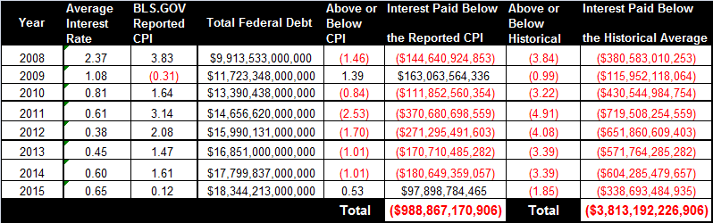
$42 billion is 4.25% of the minimum we know that savers lost in interest income from the largest negative rates of return in history for the longest period of time in history (This also assumes that you are in the 9% minority who give current BLS.GOV inflation calculations creditability).
Nearly $1 trillion confirmed in negative rates of return (below the CPI). Over $3.8 trillion relative to the 1957-2007 positive rate of return average. Source: Federal Reserve
In reality it’s likely far worse than a total of $3.8 trillion
91% of professional traders surveyed believe inflation is being under reported, 63% believe true inflation is twice what is reported. Pre-1980 BLS.GOV inflation calculation methods measure a constant standard of living; current methods measure a minimum standard of living. 1980 pre-revision BLS.GOV calculation methods put inflation three times higher than what is currently reported by the BLS.GOV.
The CPI not only dictates Treasury rates, but all other governmental expenditures that are linked to the CPI rate like Social Security benefit increases.
From 2008 to 2015, an average of $1.2 trillion has been removed from the economy annually due to lost interest income on US Treasury debt and increases that did not occur to Social Security recipients directly as a result of the current inflation misrepresentations by the BLS.GOV. Details, all supporting charts and data:
How does striping savers, Social Security recipients, soldiers, policemen, firemen, every other government employee, their suppliers and the free market out of trillions “stimulate an economy”?
What did economic stimulus do for borrowers?
In 2009, the Fed Funds bank borrowing rate dropped to 0.13%,
the prime rate remained unchanged at 3.25% until December 2015, then bumped up to 3.50%, and
consumer credit card rates remained above 13.00%, close to the 20-year average of 14.22%.
Fed Funds bank borrowing rate (red) relative to bank lending rates:
Red = Fed Funds bank borrowing rate Black = Prime lending rate Green = Average credit card rate Blue = 30-year conventional mortgage rate Source: Federal Reserve
Not that Japan is any example to follow, but when Japan’s deposit rates went to zero, the Japanese at least had the conscience to lower their prime lending rate to 0.95%
At 0.95%, Japan’s prime rate is less than 1/3 of the 3.00% gross profit margin between the US Fed Funds rate and prime lending rate.
Enabled the Treasury to finance over 10 trillion in new deficit spending at the lowest rates in history.
Allowed the US Treasury to refinance existing Federal debt at the lowest rates in history (Maturity Extension Program).
Locked in the US Treasury’s debt service cost at the lowest rates for the longest period of time in history; the average US Treasury duration is now nearly six years, and average yield less than 2.75%.
Red = Federal debt
Blue = Federal debt held by Federal Reserve banks
Light Blue = Social Security
Green = Federal debt service cost that the Fed stopped reporting Source: Federal Reserve
What “economic stimulus” did for the US economy
The US debt to GDP ratio is currently the worst since World War II at 105% and is quickly closing in on the all-time high of 113%.
Current debt-to-GDP ratio, 105%
Debt to GDP in 2009 when “economic recovery” officially began, 80.10%
Debt to GDP at the height of the Great Depression, 39%
All-time high debt to GDP during World War II, 113%
Budget deficits still exceed $400+ billion annually. Each 1.00% increase in debt service will add $192 billion to the current $400+ billion annual deficits.
The tax receipt growth to Federal debt ratio is by far the worst in history. From 2008 to 2015, the US national debt increased by 104% while tax receipts increased by only 36%.
If rates rise, it will crush tax receipts and eventually generate new high annual budget deficits.
Red = National debt
Green = Debt service cost
Black = Personal income tax receipts
Blue = Corporate tax receipts
The worst debt to personal income ratio in history
Red = National debt
Green = Personal incomeSource: Federal Reserve
The worst debt to employed population ratio in history.
Red = National debt
Green = Non-farm payroll
Black = Total population Source: Federal Reserve
Millions in the US annually are still losing their homes.
US Mortgage delinquency rates remain at 6.16% in 2016
6.16% is nearly twice the pre-recession all-time high of 3.36%
Nearly three times the pre-recession average of 2.24%
Home ownership in the 21st century is at a new all-time low. Source: Federal Reserve
The worst trade deficits on record; over $5 trillion has left the US for foreign shores since “economic stimulus and recovery” began.
From 1960 to 2007, the cumulative trade deficit was $7.73 trillion
From 2008 to 2016, $5.13 trillion
Cumulative total increase from 2008 to 2016 66.31%
Since 1960, $12.86 trillion in wealth has transferred from domestic to foreign accounts. Source 1960-2013 Federal Reserve Source 2014-2016 Trading Economics
“Quantitative Easing,” which leads to inflation and dollar devaluation.
“Quantitative Easing” created $4.19 trillion with keypunch entries backed by no tangible assets or income flow to:
Bail out the banks that facilitated the debt crisis.
Purchase record amounts of US Federal debt that no one else would buy at non competitive interest rates.
Force and hold rates at historic lows enabling the US Treasury to finance over $10 trillion in new Federal debt at the lowest rates in history.
$4.19 trillion is nearly five times greater than total Federal debt was during the “inflationary debt crisis” of 1980 when short-term rates soared above 18%.
During “economic stimulus and recovery,” the USD had an overall depreciation of 10.27% against the Chinese renminbi despite massive intervention by the Chinese to devalue their currency. Source: Federal Reserve
The World Bank tells us China’s economy will surpass the US’s by 2019.
Greenspan enabled the financial crisis
Greenspan’s agenda one week after leaving the Fed.
7 February, 2006, Lehman Brothers paid Greenspan $250,000 to meet with 15 of its most important hedge fund clients in Lehman’s executive dining room. Greenspan’s primary theme was the white-hot U.S. housing market was slowing down, but evidence of it would not show up statistically for several months and it could take more than a year.
Housing prices fell, global investor demand for mortgage-related securities evaporated, many of the attendees at the 7 February, 2016, Lehman Brothers dinner that negated Greenspan’s advice watched their hedge funds implode as subprime mortgage failures ignited the largest financial crisis in US history.
15 September, 2008, Lehman Brothers filed for bankruptcy; at the time, it was the largest BK in history, as its assets far surpassed those of previous bankrupt giants such as WorldCom and Enron.
In the video below Greenspan apologized for nearly two decades of failed monetary policy that put the US into the largest financial crisis in history, but kept Lehman’s 250K fee and still earns over 100K per “speaking engagement”
Bernanke made it worse
31 January, 2006, Bernanke becomes Fed chair. How could this clueless wonder calls on the market earn him the job to navigate the US out of crisis.
They didn’t, most traders I know believe Bernanke was put in because he was clueless after Greenspan get the Fed into so much trouble by essentially enabling the banking crisis.
Fed independence from the US government collapsed. The US government gave the Fed two options, do exactly what you’re told or we’ll audit you for the first time in 102 years. An audit would pull your alumni off the 25K to 250K per hour speaking tour and onto the jail tour. Bernanke assumed the position for the Federal Treasury rather than the Federal Justice System and currently receives 100K to 250K an hour on the speaking tour.
Now Grandma Yellen has assumed the position and is doing exactly what she is told by the federal Government telling economic recovery fairy tales that no one believes.
Fed creditability with the market is at a new all-time low
Yellen’s latest fairytale tells us the economy is in “recovery,” and there will be eight rate hikes between now and December 2018; the market says less than two.
A-C on the chart below shows the market’s expectations for rate hikes:
A) In June 2011, the market was pricing in three 0.25% rate hikes by March 2019, with the spread between the September 2016 (GEU16) and March 2019 (GEH19) deliveries at 0.75, position value at $1,875.
B) By November 2013, optimism for US economic recovery and rate normalization peaked with the market pricing in nine 0.25% rate hikes, the spread moved to 2.25, position value $5,625.00 USD.
C) Current rate hike expectations have dropped to less than two 0.25% hikes, with the spread at 0.3750, position value at $937.50.
D) If the market had faith in the Fed, the spread between the September 2016 (GEU16) and March 2019 (GEH19) deliveries would be 2.25, reflecting the Fed’s expected eight 0.25% hikes; position value $5,625.00.
E) I think the Fed is lying about the economic recovery and rate hikes while the market is overly pessimistic (basically it’s telling you to move down into the bunker). I believe we’ll see four 0.25 rate hikes between now and March 2019. I’m in this position at 0.3750 position value $937.50, my objective is 0.8750 position value $2,187.50quotes. I believe the rate hike won’t be generated by “economic recovery,” but the US’s inability to borrow as it fires up more QE and its debt creditability erodes. Give new meaning to the phrase “collateral damage” (as in borrowing collateral):
The only way the US can fix its debt problem with more debt is if the money borrowed goes to programs like Roosevelt’s which injected money directly into the economy.
1933 economic stimulus per capita; $746 or $13,785 in 2016 dollars
1933 to 1939, the Federal debt-to-GDP ratio moved from 39.40% to 43.25%
1939 national debt per capita $663 or $11,458 in 2016 dollars
Obama’s stimulus injected money directly into the banks that caused the problem, and pork programs at the same, it removed money from the economy through negative rates of return and BLS.GOV inflation misrepresentations.
2009 economic stimulus per capita; $2,691 or $3,003 in 2016 dollars
2008-2016 Bank bailouts already paid per capita $14,426
2008 to 2016, the Federal debt-to-GDP ratio moved from 67.85% to 105.20%
2016 national debt per capita $60,215
2016 total bank bailouts guaranteed by the US government $52,688 per capita
Trying to fix a bad debt problem with an even greater bad debt has and never will work.
Hopefully, the FOMC will figure outBanqiao bankingjust doesn’t work andmisreporting inflationmay work in the short term, but will have horrific long-term consequences.
FOMC voting members who determine monetary policy and set rates for the United States
Enough of the bad news
The good news is the bad news generates major market moves and powerful trends. It’s going to be a fun year for traders who are on their game and have strategies in place to capture them.
If Greece, a country with a GDP the size of Orange County, California, or the UK (3.94% of global GDP), can generate the moves we’ve seen, just think of how much fun we’re going to have in the US markets (23.32% of global GDP) with the kind of fundamentals we have and an election year on deck.
My purpose in writing these long-winded articles is so I can reference them on this site over the next year as I write about specific trades in shares, indices, debt instruments, currencies, metals and energies.
I think it’s time for all to brush on the sectors you’ve forgotten about, your shorting and collar strategies. Metals are sure to shine, debt instruments look like they be a downer (rates higher), and we should have the opportunity to pick up our favorite US shares at much better prices after the selling hemorrhage stalls.
Few of my favorite US stocks and ETFs I’ll be writing about use my own trades as examples (both short and long). If there is interest, I’ll expand to international markets.
Volatility will be high, so trade with the trend; when possible, use option collars to define your risk on trades and for the duration of every trading period.
I run a family office from the Virgin Islands, have about 1/3 of assets in US markets and like to get some online international camaraderie going as we batten down the hatches getting ready for the next leg of this adventure.
I have been a professional trader for over 20 years including time on the floor. My sole professional purpose is the preservation and enhancement of family wealth. I don’t sell a newsletter, I don’t manage US funds (only non-US), but I do enjoy trading the liquidity of US markets, especially on days like Brexit.
Good luck, America. I can feel the pain and disappointment you must being going through looking at your economic numbers. I sure hope you can come up with a better line up of leaders this fall.
The expression Banqiao Banker was coined by professional traders comparing current Central Bank monetary policy to the Banqiao Dam disaster. In short you can’t fix a problem by making it larger. In the case of Central Bank policy you can’t fix a debt crisis by creating a larger debt crisis.
Correlations Banqiao Dam Disaster and Banqiao Banking Disaster
Weight of water that the dam holds
Weight of the debt that the government holds
The dam was poorly designed,hastily constructed and not safe from the start.
The US Fiat monetary system was poorly designed, hastily constructed and not safe from the start.
The Chinese Government told its citizens the solutions they implemented to resolve the problems with the dam worked.
The Fed is telling US citizens and debt investors that their economic “solutions” are working and that the US economy is in “recovery”.
Reality; the damage the dam was designed to prevent and costly solutions to repair and “improve” the dam created an even larger problem.
The costly Central Bank solutions for economic crisis are putting the global economy at far greater risk than the problems these solutions were designed to correct.
An apathetic public believes government rhetoric about the dam’s safety contrary to the facts.
An apathetic public believes government rhetoric about Inflation the Fed’s Central Bank Policies and representations of “economic recovery” contrary to the facts.
The weight of the water eventually collapses the poorly designed dam setting off a chain reaction that impacts 62 facilities down river ultimately killing over 170,000 people and destroying 5,960,000 buildings. The total carnage done by the dam’s collapse is far greater than any flood damage the dam was originally designed to prevent.
The weight of debt generated by Central Bank “solutions” could collapse the US economy setting off a global chain reaction destroying or damaging smaller economies creating an even far greater economic crisis than what Fed policy solutions are trying to correct.
Banqiao Dam Disaster
The Banqiao Dam was hastily designed by academics using hypothetical hydrology theory with less than ½ as many gates as recommended by those who had actual hydrology experience in the design and building of dams.
Those who had actual experience warned that a dam with less than half the required gates could not possibly hold up against several typhoons that had occurred during the previous 50 years. The academics dismissed those whom had actual experience as dated and insisted their dam would be stronger and last longer than those designed by the “old timers”.
The government sided with the academics and fired the “experienced old timers” as the academic’s version of the dam could be built in a shorter period of time to solve the long term problem of flooding in the Huai river basin which was very problematic in 1949 & 1950.
Construction of the Banqiao dam began in April 1951 and was completed in June 1952.
US Central Bank Policy (Banqiao Banking Disaster)
In 1971 the US decided to abolish what remained of the gold standard and make the US dollar a fiat currency enabling the Fed to “create” as much money as it needed to dam up any debt typhoons generated by Capital Hill and manage the occasional deficit flooding.
Economic Academics using hypothetical theories said it would work, economists and traders with actual work experience said it wouldn’t work.
After a series of higher than expected rainfalls in the in the 1950’s & 1960’s the Government acknowledged the Dam might have “minor” structural issues (as it was made in majority out of clay).
They told residents not to worry as the best hydrology engineers and other professionals had been deployed to resolve the structural issues with the dam.
They represented the issues had been resolved and their solutions had made the dam stronger than most, the Government renamed the Banqiao Dam to the “Iron Dam” and considered it to be unbreakable.
The Government that built the dam then appointed a team of engineers to monitor the dam the Government built.
The Government employed engineers routinely provided glowing updates on Dam’s structural integrity.
The Government sponsored monitoring team told residents there was no danger when in reality the solutions didn’t repair the dam they had made the Dam less safe, putting the complacent residents at even greater risk.
Decades after the collapse it was learned the governmental monitoring agency “revised” these updates to more accurately reflect the structural integrity of the dam.
US Central Bank Policy (Banqiao Banking)
1971 the US abandons the gold standard
1971-1979 The US had been hit hard by a series of debt typhoons causing massive deficit flooding, the national debt grew from 391 billion in 1971 to 845 billion by 1979 or +116.11%.
Buy 1979 the debt level behind the fiat monetary dam had risen above any level the dam was designed to accommodate. Cracks in its structure became unmanageable and the design flaws became very apparent.
By 1980 the warning sirens of inflation were blaring at full volume, telling investors to seek the safety of higher ground in tangible assets such as gold.
At the same time the US Government Fed, and B.L.S. told investors not to worry about the structural flaws in the newly created fiat monetary system because the best financial engineers led by Paul Volker (then Fed chair) had been deployed to resolve any issues. Volker’s team made a valiant effort in vain to repair it.
The US government also told investors the Bureau of Labor and Statistics (BLS.GOV) was “at the scene”.
The US government reiterated the people of the BLS.GOV who they hired to monitor them would provide US citizens and debt holders with regular updates on the structural integrity of the 9 year old Fiat Monetary System.
The US Government at the same time told their employees at the BLS.GOV to revise their inflation calculations to more accurately report inflation. Government employees at the BLS.GOV immediately complied and implemented the largest number of revisions to the CPI calculations since the CPI’s inception in 1919. Essentially the calculations started moving from a constant cost of living Index to the minimum cost of living index.
The US Government, Fed and BLS assured investors their assets were safe despite the ever increasing debt load behind the fiat monetary system dam. The BLS.GOV using the “revised” and more “accurate” inflation reporting gave US citizens and investors in US debt a false sense of security. See Consumer Price Index fact or BLS.GOV fiction.
The US didn’t fix the inflation or debt crisis they just turned off the warning sirens of accurately reported inflation and other economic releases putting US citizens and investors in US debt at far greater financial risk.
Banqiao Dam Disaster
Typhoon Nina landed onto the scene with a bang in 1975, hitting China hard and quickly.
On the night of Aug 8, 1975, a line of people frantically piled sandbags atop Henan Province’s Banqiao Dam while being battered by the worst storm ever recorded in the region. They were in a race with the rapidly rising Ru River to save the dam and the millions of people that lay sleeping down river. It was a race they were about to lose.
Just after 1:00 am, the sky cleared and stars emerged from behind the storm clouds. There was an eerie calm as someone yelled, “The water level is going down! The flood is retreating!”
There was little chance to enjoy that calm. One survivor recalled that a few minutes later it “sounded like the sky was collapsing and the earth was cracking.” The equivalent of 280,000 Olympic-sized swimming pools burst through the crumbling dam, taking with it entire towns and ultimately hundreds of thousands of lives.
The 24.5-meter dam of Banqiao Reservoir which took the most rain from the typhoon first breached at wee hours of Aug. 8, releasing within six hours 700 million cubic meters of water that wiped Daowencheng down river from the map immediately, killing all 9,600 citizens.
“Houses and trees disappeared all in a instant. Thousands of corpses and cattle floated in water.”
To worsen the situation, the facilities of 62 reservoirs collapsed or were damamged down river one after another unleashing about 6 billion cubic meters of water over an area of 10,000 square kilometers.
Official statistics recorded 30 years latter show more than 10 million people were affected, all communication to and from the cities were cut off for months, some never restored until years latter.
The appalling images of the dams burst were not publicized during at that time. Chinese leaders considered natural disaster death tolls a state secret, an investigation by the central government soon after the floods found a series of “unexpected structural failures” that led to the disaster.
Li Zechun, who first arrived at the scene (now the Chinese Academy of Engineering Sciences) qualified the tragedy “as a man-made calamity rather than a natural one.”
Li said the water storage for irrigation function of a reservoir was overemphasized amid reservoir construction despite warnings by scientists that much of a reservoir’s flood control was inadequate .
The Banqiao Reservoir was designed with a capacity of only 492 million cubic meters but it had to accommodate more than 700 million cubic meters of floods and it has less than half the recommended gates.
The dam collapsed killing approximately 26,000 people from the initial flooding and another 145,000 during subsequent epidemics and famine. 5,960,000 buildings collapsed, 10 million residents were affected. Unofficial estimates of the number of people killed by the disaster have run as high as 230,000.
US Central Bank Policy (Banqiao Banking)
The Fed’s collsal experiment based on hypothetical academic theory and assumptions Led by Alan Greenspan enabled the crisis.
Greenspan apologizes for his decades of failied Fed policy in this short video.
Then the unproven solutions that Bernanke implemented made the crisis multiple times worse and did irreparable damage.
How could Bernanke with his bio and bad calls on the economy ever have be appointed Fed chair as the US faced its debt crisis?
His Bio and calls on the economy
Now Grandma Yellen tells an apathetic US population economic recovery fairy tales while the 45 year old fiat monetary dam holding back unknown trillions in debt and unfunded liabilities is cracking hard, right down the middle.
Beyond repair
Red = Federal debt
Green = Debt service on the national debt
Blue = Debt held by Federal Reserve Banks
Black = Federal government receipts from personal taxes
Grey = Federal government receipts from corporate taxes
Are we really supposed to believe this fester of Central Bankers (FOMC voting members) made up mostly of Academics with very little private sector actual work experience will lead the US out of its biggest financial crisis in history?
I run a family office from a beautiful tax free Caribean Island, I’ve been a professional trader for over 20 years including time on the floor. My sole professional purpose is the preservation and enhancement of family wealth. I don’t sell a newsletter, I won’t manage a penny of US investor money but I do enjoy trading US markets especially on days like Brexit.
The gains we make on the moves generated by events such as Greece or Brexit would be a whole lot more rewarding if they we’re generated by good news rather than bad and we didn’t have to worry about preservation of the money we make on the back end.
Watching the US and european financial systems in a death spirale, the jeopardy current Central Bank policies is putting our US assets in, the potential of these policies setting off a chain reaction impacting our Global assets is more than disturbing
I should be getting drunk and chasing sea turtles with my beautiful wife but at the beach but nooooo, I’m stuck here in my office, buying metals like I’m going to live in a bunker for the rest of my life. I’m working like a galley salve on collaring up my long positions, defining what short positions I’ll be taking next, and when as the current collection idiots tries to figure out you can’t solve a debt problem by creating an even bigger debt problem.
I know the US is becoming more 420 friendly but it appears to me the FOMC members are abusing 24% cannabis while on the toilet, getting so high that they’re flushing ethics, responsibility and common sense down the toilet and what should have been flushed ends up being their decisions.
From their pictures it looks to me like they just can’t handle those 24% Indicas, maybe they should try some milder 4-6% Sativas? I have yet to develop a taste for cannabis but I may have too after their monetary policies banish me to the bunker so I can kill the boredom while I polish my guns before the big rat hunts so I can feed my family.
America
Please elect leadership that has a backbone and can make responsible decisions. Trump with his temper/business failures and Hilary Clinton who couldn’t even keep an eye on her own husband is the best you can do?
What ever happened to leaders like Franklin Roosevelt not only did he put millions of Americans back to work rebuidling the infrastructure of the United States he delt with Hiltler, Mussolini and Hirohito and they prepared to try and take over the entire world.
Please find a leader like F.D.R. audit the Fed for the first time in its 102 year history, trash the BLS.GOV and replace the BLS.GOv with a totally indemendant agency that will generate actual economis data (what a concept) . Hold those that created this debt mess responsible, taking vile little vermin like Greenspan and blowhard Bernanke off the 100K to 250K dollar an hour “lecture tour” and onto the jail tour.
All the money the “Quantitative Easing” printing press can print up, all the BLS.GOV revision magic they can dream up, all of Grandma’s Yellen’s economic recovery fairy tales can’t repair the US debt damage, its stage 4, the dam has cracked right down the middle, the charter builder and financial hemorrhage are dead on th horizon
If Greece with an economy the size of Orange County California or the UK (3.94% of the global economy) abandoning a sinking EU ship can rattle the markets, just imagine when the fertilizer hits the fan in the US representing 23.32% of the global economy.
Sure it’s going to be a lot of fun to trade the major market moves that will be generated, sure we stand to enhance our fortunes, but I for one would rather make money off of good news than economic misery fueled by surfeit of politicians and intrusion of miscreant Central Bankers.
Quotes for the day
Suppose you were an idiot. And suppose you were a member of Congress. But I repeat myself. – Mark Twain
In my many years I have come to a conclusion that one useless man is a shame, two is a law firm, and three or more is a congress. – John Adams
Less than 9% of professional traders surveyed give the current C.P.I. releases credibility. 91% believe the actual C.P.I. is higher, 63% believe the CPI is more than twice reported C.P.I.
What the C.P.I. is used for
Since 1919 the CPI has been used as a benchmark to set US Treasury deposit rates.
The C.P.I. is also used in Adjusting Income and Payments for Government Expenditures; Social Security beneficiaries, Military, all Government Employee salaries, welfare, food stamp recipients, Governmental rents, nearly everything right down to school lunches.
Since 1978 there has been justifiable controversy about the creditability of the C.P.I. currently B.L.S. creditability is at a new all time low.
Fact or fiction?
Let’s compare current “revised and weighted” BLS.GOV C.P.I. calculations to the constant pre 1980 calculations for;
Predicting the price for gold from 1971 to 2015
Governmental expenditures 1978 to 2015
Gold
In 1971 the US abandoned the US dollar’s peg to gold, gold was trading at $40.80.
Current BLS.GOV C.P.I. calculations
According to 618 million dollars in annual BLS.GOV funding the price of gold should have risen from $40.80 in 1971 to $238.77 by 2015.
Use the BLS.GOV inflation calculator on this page enter the data below.
Actual price of gold for 2015, $1,159.82
Current calculations are off by $921.05 per ounce.
Pre 1980 BLS.GOV C.P.I. calculations
The price of gold should have been $1,1104.78 in 2015.
Actual price of gold $1,159.82.
Pre 1980 calculations were off by $55.05 per ounce for the 45 year period.
$55.05 per ounce is slightly greater than the most recent 5 day range for gold of $41 and less than half the most recent 1 month range of $125.
Prior to doing the numbers on Governmental expenditures lets look at the demise of C.P.I. creditability and why.
In 1969 Federal debt service cost began to outpace Federal tax receipts, by 1971 the debt service cost/tax receipt ratio was considered “unmanageable”.
To resolve this problem in 1971 President Richard Nixon (prior to his impeachment hearings), then Fed chair Arthur Burns along Paul Volcker abandoned the gold standard.
The US dollar officially became a Fiat currency enabling the US’s private Central Bank to create as much money as the US Treasury needed (at their unaudited discretion) to satisfy the Treasury’s debt addiction.
The US had two choices
1) To change course and use the ability to create money to bridge deficit gaps until the causes of the deficits could be discovered and resolved.
2) To maintain its course indulging in short-term monetary gratification with complete disregard of the long-term consequences, dollar valuation, inflation or future generations.
Unfortunately, the US chose option # 2, budget deficits soared and the national debt grew from 391 billion in 1971 to 845 billion by 1979 or +116.11%.
Predictably, the creation of massive amounts of money backed by no tangible assets or income flow generated U.S. dollar devaluation and double-digit inflation.
U.S. Federal debt service cost and all other Governmental expenditures skyrocketed generating a population adjusted per capita increase in Federal Spending of 156.38% for the 9 year duration of the US’s newly created “fiat currency“.
Even with the minor modifications that had been made to the B.L.S. C.P.I. calculations “to more accurately report inflation” the B.L.S. calculations show an increase of 124%.
By 1980 the US dollar looked doomed, nearly every tangible asset on the board rallied against the US dollar, speculation frenzied, 100’s of millions were being made and lost in minutes.
Gold and silver moved sharply higher, bullion banks were facing “fails to deliver“. Bankers, the Fed, US Treasury, Bureau of Labor and Statistics, exchanges and Global Investors were in panic mode.
36 years ago the US Treasury, BLS.GOV and Fed still had a shred of conscience. PaulVolcker the newly appointed Fed chair began a series of very aggressive rate hikes to contain inflation.
At the same time the B.L.S. was given the “all clear” by their employer (The U.S. Government) to use “revisions” more aggressively “to more accurately report US inflation and employment”.
By 1983 Volcker was hailed as a hero because the cumulative impact of his tight monetary policies and BLS.GOV inflation calculation magic had dropped the reported BLS.GOV inflation from its peak of nearly 15% in 1980 to under 3% by 1983.
This video tells the story in 2 1/2 minutes
The market’s reaction shows the impact
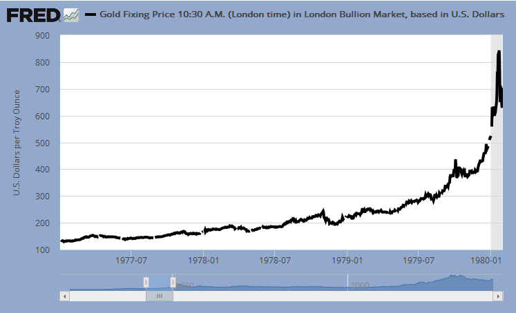
A) 1979 Volcker begins a series of aggressive rate hikes, the yield curve inverts. (short-term rates exceed long-term rates)
B) 1980 higher rates “revised” BLS.GOV inflation calculation magic fully engages, the initial reaction is muted at first as the market just doesn’t believe it.
C) In 1983 after more than a decade of high inflation it magically lowers from near 15.00% to less than 3.00% containing Federal debt service cost and all increases in governmental expenditures that are linked to the “official” CPI such as Social Security.
What the market didn’t pay attention to in 1980 and still isn’t in 2016 are the major revisions to the way that the C.P.I. is being calculated or the impact of BLS.GOV revision magic to U.S. citizens, U.S. debt holders or the motivation for the revisions.
The Consumer Price Index (C.P.I.) was created to help businesses; individuals and government adjust their financial planning for the impact of inflation.
Let’s do the math and compare BLS.GOV inflation calculations to actual price increases from 1978 to 2015.
Actual Federal Spending per capita for 1978 was $2,093.02
Using BLS.GOV inflation calculation methods, posted on the BLS.GOV website, per capita Federal spending should have increased from $2,093.02 in 1978 to $7,068.61 by 2015 or up 273.15%
Actual Federal spending per capita in 2015 was $11,339.23 or up 456.11%, the BLS.GOV again is off this time by 182.96%
This 456.11% increase was contained by the BLS.GOV understating inflation and short-changing 100’s of millions of Savers, Pensioners, US Soldiers, families of fallen Soldiers, Policemen, Firemen, Teachers all other Federal Employees and Governmental suppliers out of trillions of dollars to save their employer the US government the same.
There is no conscience in the Treasury.GOV and BLS.GOV game.
You can take nearly any period on anything from home prices, oil, food, college tuition stocks or funeral costs and the BLS.GOV calculations on this page will underestimate the actual increase by a significant amount.
Facts
BLS.GOV revision magic saved the U.S. Treasury over 1.5 trillion in 2015, just in debt service cost and pensions alone.
Below the last 20 years for debt service cost and pensions (without compounding)
BLS.GOV revision magic has saved their employer the U.S. Treasury on average 1/2 a trillion per year versus the pre 1980 BLS.GOV C.P.I. calculation methods.
Measurement of consumer inflation traditionally reflected measuring the cost of maintaining aconstant standard of living, as measured by a fixed-basket of goods.
The changing costs of maintaining a constant standard of living were measured by pricing out a fixed-basket of goods and services-same components, same weighting-period after period.
Whatever the percentage change was in the cost of that basket of goods that is how much income would have to rise in order for someone to maintain a fixed or constant standard of living over the given period.
Tracking changes in the cost of a fixed basket of goods was the approach to estimating inflation, going back to at least the 1700s. Prior to 1945, the fixed-basket CPI tracked by the U.S. government was known as the Cost of Living Index.
It assumes you
Lived in the same size home
Ate the same food
Used the same amount of Energy
Your children attended the same schools
Had the same medical coverage
Bought the same brand of drugs
You drank the same amount and brand of Alcohol
Ate at the same restaurants
Attended the same type of theatrical productions
Drove the same type of car
You had the same household staff that worked the same hours
You get the idea; it was a fixed basket measuring the cost of a constantstandard of living
The way it is now
The CPI now consists of more than 80,000 items in over 200 categories arranged into eight major groups, “Hedonic Quality Adjustments“ are applied then the data is “weighted” to reflect a “more accurate” representation of inflation.
Are you kidding me? I don’t think I’ve purchased 80,000 different items in my entire life.
Current calculations allow substitution of lower-priced and lower-quality goods in the basket (i.e. replacing château Laffite Rothschild with Boones Farm wine you’re still getting a bottle of wine, it does the same thing, so there is no change in price that impacts inflation) It actually can lower the reported rate of inflation versus the fixed-basket measure.
Geometric weighting; a purely a mathematical gimmick that automatically reduces the weighting of goods rising in price, and vice versa, it has no demonstrated relationship to consumer substitution of goods based on price changes. It was explained as a surrogate for a substitution measure.
More frequent re weightings of the CPI index from every ten years to every two years, which moved the CPI closer to a substitution based index, but the change was not considered a change in methodology.
Ongoing re-weightings of sales outlets, also moving closer to a substitution-based index and creating other constant standard of living issues. If you can no longer afford your tailor you can by your clothes at K-mart, you’re still getting a pair of slacks so you’ve helped inflation moved lower.
“Hedonic” quality adjustments, altering the pricing of goods and services for nebulous quality changes that could not be priced directly and that often are not viewed or recognized by the consumer as a desired improvement. (You buy a new boat, it’s the same length and power as your old boat but it costs 50% more, according to the BLS.GOV your new boat is going to last twice as long therefore the price has actually gone down).
It just goes on and on and on, the excuses and justification for revisions are just beyond pathetic. What these revisions are doing to Pensioners, Savers, Federal employees is beyond criminal.
There is only one reason the BLS.GOV “revisions” are in place and 92% of us know it, it’s to save their boss the Treasury.GOV trillions at the expense of US citizens and debt investors.
Sure we’ve all made money on their misrepresentations but I’d rather be reviewing quality long-term positions rather than trying to profit from their next lie.
I run a family office from a tax-free spec of an island 1,770 kilometers south-east of Palm Beach Florida. As the head of a family office my sole professional purpose is the preservation and enhancement of family wealth.
The recession may be technically over but its effects on our life and language are far from it. In fact, some recession words have become so ubiquitous – staycation, for one (see below) – that they just might be here to, ahem, stay.
Recession language isn’t a new phenomenon. Thanks to the Great Depression we have terms like: Okie, dirt poor, and baloney (to mean ridiculous, not the mystery sandwich meat). Even the term “depression” has been attributed to Herbert Hoover, who is thought to have wanted to avoid using the more common, but more alarming terms “panic” or “crisis” to describe what subsequently became known as the Great Depression.
So, in the spirit of trying to laugh at our collective condition, we’ve compiled a lexicon of our Top 10 favorite words birthed by the recession. Laugh, cry, and submit your favorite new-economy words in the comments below.
Recession slang: 10 new terms for a new economy
10. Funemployment, n. The practice of enjoying one’s unemployment.
The funemployed subscribe to the philosophy that in the face of bleak employment prospects, it’s better to make the most of time off by catching up with old (read: also unemployed) friends or developing low-cost hobbies, ideally during normal business hours to realize the additional benefit of irking ones employed friends.
Sample sentence: As part of my funemployment plan, I’ve joined an Ultimate Frisbee league and am providing foster care to three puppies.
See also: Funderemployed (adj.) taking a job that’s fun because employment that pays well or is in one’s field is unavailable.
9. Insource, v. To do oneself what one previously paid others to do.
Sample sentence: “No, I can’t meet you for brunch this morning. I’m insourcing my laundry these days and have five loads piled up.”
Alternate sample sentence: “I know my nails look like someone took a chainsaw to them, but I insource manicures now.”
Antonym: outsource.
8. Staycation, n. Vacationing at home or near home because traveling further would be prohibitively expensive.
For better or worse, staycation is perhaps the most widely-used and accepted term of the new-economy lexicon.
Sample sentence: “That’s right, if something doesn’t change, we’re going to have to staycation at my in-laws this summer … again.”
7. Intaxication, n. A sense of delight mingled with the perception of instant wealth that one feels upon receiving a tax refund.
Sample sentence: “It seemed like a good idea to charge that pair of Louboutins/small boat/Caribbean vacation to my credit card when I got my tax refund. But when I got my statement a week later, it was clear I was in a haze of intaxication at the time of purchase.”
6. Madoff’d, v. To get ripped off in a particularly offensive fashion.
Sample sentence: “Oh man, that cab driver totally Madoff’d me. I gave him a $20 and he only gave me change for a $10.”
5. Recessionista, n. A consumer who has historically paid big bucks to look like a million bucks and who, unwilling to quit his/her fashion habit in the face of the recession, has found alternative ways to maintain a certain standard of wardrobe.
Such strategies often include shopping at discount and second-hand stores. More prevalent in the media than in everyday conversation.
Sample sentence: “The clerks at Barneys are suffering from withdrawal now that I’m a recessionista and rent my handbags online instead of buying.”
4. Mancession, n. A recession, such as this most recent one, which hits men harder than women.
Sample sentence: “The extent of this mancession became clear to me when I realized it was all dads in F-250s in the carpool line.”
See also: he-cession.
3. Povo, adj. A two-syllable “abbreviation” for poor, often with a mocking or self-defacing tone that lacks any serious derision or the class implications associated with “poor” or “poverty.”
Derivation: Australian (Aussie) English
Sample sentence (better if said with faux Australian accent): “We’re living sans Internet and cable now that my povo roommate won’t chip in for it anymore. It’s like the 1980s around here.”
2. Permatemp, n. The condition of being permanently employed as a temporary worker.
This could be due to lack of motivation to seek permanent employment, inability to find permanent employment, or the permatemp’s belief that a company will eventually hire him/her for the job s/he is currently doing for lower pay and without benefits.
Sample sentence: “Wake up, Joe. You’ve been here for six months, your cubicle is decorated better than your living room, and the hiring manager still doesn’t know your name. You’re officially a permatemp, my friend.”
1. Decruited, adj. To be fired from a position one has not even started yet.
Sample sentence: “At first I felt really bad about being decruited from that corporate law firm after spending two summers of law school interning for them. But then I decided to make the most of my funemployment and use my signing bonus to travel around Europe.”
The last major silver short squeeze was in 1980. During the squeeze, the New York and Chicago exchanges halted silver trading several times. Whenever markets were disrupted, the price quoted in New York did not match the price buyer had to pay for the actual silver.
Premiums above the spot price for silver got very high – as much as $10 per Troy ounce. However, people were happy to pay the high premiums, and glad to get silver in almost any form. Customers were not concerned about brands, shapes, or sizes of silver bars, or denominations of U. S. 90% silver coins. They just wanted silver.
S T A G F L A T I O N
America was almost in a depression during the 1970s. Economists called it stagflation. We had high unemployment and sky-high fuel costs. And, inflation was terrible. The U. S. economy was in pretty bad shape; but not in the shambles it is now.
After the U. S. abandoned a gold standard in 1971, people began buying gold and silver coins to protect themselves from the dollar’s loss of purchasing power. Most coin and bullion buyers weren’t looking for paper dollar profits. They wanted tangible assets to hedge against a crumbling dollar.
T H E L A S T M A J O R S I L V E R S H O R T S Q U E E Z E
Silver was $1.95 per ounce in the early 1970s, when Nelson Bunker Hunt, William Herbert Hunt, and other wealthy investors began accumulating physical silver. They informed the public they would be systematically building physical positions in silver. Over a period of years, silver moved from $5 to about $11 per ounce mid-1979. Silver was more than $30 per ounce at the end of 1979.
The Hunt brothers’ long position was 100 millionounces of silver. On each delivery month, the Hunts and other investors paid off their contracts and were taking delivery of the silver (5,000 ounces of silver per contract). Until then, there never had been so much demand for so much physical silver on the exchanges. *
As silver began moving sharply up in 1979, the bullion banks were facing “fails to deliver” on their open contracts. It was rumored nine directors of the COMEX held massive short positions in silver. The situation was called a silver short-squeeze. At the end of the squeeze, the market was near collapse and the shorts were almost broken. The short squeeze threatened the very viability of the exchange. The rules for trading silver on the COMEX (Commodities Exchange New York) and CBOT (Chicago Board of Trade) were changed many times until the squeeze came to an end.
W H E N T H E E X C H A N G E S H A L T E D S I L V E R T R A D I N G
The exchanges stopped trading silver several times during the silver short squeeze (and during its aftermath). There were “limit up” days, “limit down” days, and “liquidation only” days. There was uncertainty in the exchanges, tremendous price volatility, and extraordinarily wide spreads (big percentages between bid and ask). Locking in prices over the phone became risky for customers, wholesalers, and dealers.
In those frantic days, people stood in lines half-way around city blocks at coin shops throughout the country, hoping dealers would not run out of silver. People even traded with each other while standing in lines. Supplies of silver bars and silver coins were strained to the breaking point.
C O M E X S I L V E R : L I Q U I D A T I O N O N L Y
Time after time, exchanges such as the COMEX and the CBOT raised margin requirements in an attempt to drive the price of silver down, and make it too expensive for investors to stay “long” in the silver market.
Then, they limited the number of contracts investors could buy. In New York, customers were limited to 10 million ounces of silver; the CBOT put on a limit of 3 million ounces. In March 1980, the CFTC (U. S. Commodity Futures Trading Commission) finally broke the back of the silver short squeeze.
Silver was on its way to $50/oz. The final game rule was changed to stop the price advance. The CFTC banned all purchases of silver contracts, allowing liquidation only.
Silver tumbled 50% in four days.
The total decline was 78% in two months.
After the silver market plummeted, it remained in the tank for more than twenty years. The shorts made fabulous profits. And, those on the other side of the trade lost their shirts. With the price of silver in the $20s, the Hunts were unsuccessful in their efforts to raise capital to pay margin calls. The Hunts declared private bankruptcy in 1980. In the end, Hunt liabilities were $2.5 billion and their assets had been reduced to $1.5 billion.
The Hunt brothers were not big enough
to fight the financial insiders bankrolled
by the Federal Reserve; or powerful enough to counter the actions of the CFTC.
In August 1988, the Hunts were convicted and heavily fined for “conspiring to manipulate the market.”
The Hunt brothers were not the conspirators. They were the victims of the same short-sellers who manipulate the prices of precious metals to this day.
PROGRAM AVAILABILITY IS DEPENDENT ON YOUR COUNTRY OF RESIDENCY AND FINANCIAL STATUS
PAST RESULTS ARE NOT NECESSARILY INDICATIVE OF FUTURE RESULTS. EXAMPLES OF HISTORIC PRICE MOVES OR EXTREME MARKET CONDITIONS ARE NOT MEANT TO IMPLY THAT SUCH MOVES OR CONDITIONS ARE COMMON OCCURRENCES OR ARE LIKELY TO OCCUR.
HYPOTHETICAL PERFORMANCE RESULTS HAVE MANY INHERENT LIMITATIONS, SOME OF WHICH ARE DESCRIBED BELOW. NO REPRESENTATION IS BEING MADE THAT ANY ACCOUNT WILL OR IS LIKELY TO ACHIEVE PROFITS OR LOSSES SIMILAR TO THOSE SHOWN IN FACT, THERE ARE FREQUENTLY SHARP DIFFERENCES BETWEEN HYPOTHETICAL PERFORMANCE RESULTS AND THE ACTUAL RESULTS SUBSEQUENTLY ACHIEVED BY ANY PARTICULAR TRADING PROGRAM. ONE OF THE LIMITATIONS OF HYPOTHETICAL PERFORMANCE RESULTS IS THAT THEY ARE GENERALLY PREPARED WITH THE BENEFIT OF HINDSIGHT.
IN ADDITION, HYPOTHETICAL TRADING DOES NOT INVOLVE FINANCIAL RISK, AND NO HYPOTHETICAL TRADING RECORD CAN COMPLETELY ACCOUNT FOR THE IMPACT OF FINANCIAL RISK IN ACTUAL TRADING. FOR EXAMPLE, THE ABILITY TO WITHSTAND LOSSES OR TO ADHERE TO A PARTICULAR TRADING PROGRAM IN SPITE OF TRADING LOSSES ARE MATERIAL POINTS WHICH CAN ALSO ADVERSELY AFFECT ACTUAL TRADING RESULTS. THERE ARE NUMEROUS OTHER FACTORS RELATED TO THE MARKETS IN GENERAL OR TO THE IMPLEMENTATION OF ANY SPECIFIC TRADE PROGRAM WHICH CANNOT BE FULLY ACCOUNTED FOR IN THE PREPARATION OF THE HYPOTHETICAL PERFORMANCE RESULTS AND ALL OF WHICH CAN ADVERSELY AFFECT ACTUAL TRADING RESULTS.
BID/ASK SPREADS, BROKERAGE COMMISSION, CLEARING, EXCHANGE AND REGULATORY FEES WILL HAVE AN ADVERSE IMPACT ON THE NET OVERALL PERFORMANCE OF YOUR ACCOUNT. PRIOR TO MAKING A DECISION TO PARTICIPATE IN ANY INVESTMENT MAKE SURE YOU FULLY UNDERSTAND THE FEES ASSOCIATED WITH TRADING.
THE INFORMATION PROVIDED IN THIS REPORT CONTAINS RESEARCH, MARKET COMMENTARY AND TRADE RECOMMENDATIONS. YOU MAY BE SOLICITED FOR AN ACCOUNT BY ONE OF OUR REPRESENTATIVES OR EMPLOYEES. IT SHOULD BE KNOWN THAT THE REPRESENTATIVES OF OUR FIRM MAY TRADE FUTURES AND OPTIONS FOR THEIR OWN ACCOUNTS OR THOSE OF OTHERS. DUE TO VARIOUS FACTORS (SUCH AS MARGIN REQUIREMENTS, RISK FACTORS, TRADING OBJECTIVES, TRADING INSTRUCTIONS, TRADING STRATEGIES, AND OTHER FACTORS) SUCH TRADING MAY RESULT IN THE LIQUIDATION OR INITIATION OF FUTURES OR OPTIONS POSITIONS THAT DIFFER FROM THE OPINIONS AND RECOMMENDATIONS FOUND IN THIS REPORT.
PAST PERFORMANCE IS NOT NECESSARILY INDICATIVE OF FUTURE PERFORMANCE. THE RISK OF LOSS IN TRADING FUTURES CONTRACTS OR COMMODITY OPTIONS CAN BE SUBSTANTIAL, AND THEREFORE INVESTORS SHOULD UNDERSTAND THE RISKS INVOLVED IN TAKING LEVERAGED POSITIONS AND MUST ASSUME RESPONSIBILITY FOR THE RISKS ASSOCIATED WITH SUCH INVESTMENTS AND FOR THEIR RESULTS.
YOU SHOULD CAREFULLY CONSIDER WHETHER SUCH TRADING IS SUITABLE FOR YOU IN LIGHT OF YOUR CIRCUMSTANCES AND FINANCIAL RESOURCES.
Expect a maximum of 3, 0.25% rate hikes by December 2018
Rates will not “normalize” this decade
True economic recovery will take far longer than than the most pessimistic of Fed guesstimates.
A-C on the chart below shows the markets expectations for rate hikes
A) In January 2013 the market was pricing in 6 , 0.25% rate hikes by December 2018, with the spread between the June 2016 (GEM16) and December 2018 (GEZ18) deliveries at 1.50, position value 3,750.00 USD
B) By November 2013, optimism for US economic recovery and rate normalization peaked with the market pricing in 10, 0.25% rate hikes with the spread at 2.50, position value 6,750.00 USD
C) Current rate hike expectations have dropped to less than 3, 0.25% hikes, with the spread at 0.6250, position value 1,562.50 USD
D) If the market had faith in the Fed’s projections the spread between the June 2016 (GEM16) and December 2018 (GEZ18) deliveries would be 2.50 reflecting the Fed’s expected 10, 0.25% hikes, position value 6,250 USD.
To convert the contact delivery price into rate it represents take 100.00 – contract price = the rate.
Example, 100.00 – the December 2016 contract price of 99.17 = an expected rate of 0.83%.
To calculate expected rate increases between delivery months take the nearby delivery minus the forward delivery equals the expected rate change between the delivery months.
Example, June 2016 delivery trading at 99.3350 – December 2016 at 99.1700 = the expected increase in rates from June 2016 to December 2016 = 0.1650%.
What U.S. price action tell us.
The market’s perception of economic recovery is far worse than the Fed’s.
Rates will not “normalize” during this decade.
Fed and US fiscal policy makers creditability with the market is at a low
Eurozone market expectations are worse.
A) In January 2013 the Eurozone expected an increase in the 3 month Euro Interbank Offered Rate (EuriBor) between June 2016 (IMM16) and December 2018 (IMZ18) of 0.6000%, position value 1,500.00 EUR
B) By November 2013 optimism for Eurozone economic recovery and rate normalization peaked with an expected increase in the EuriBor rate between June 2016 (IMM16) and December 2018 (IMZ18) of 1.10%, position value 2,750.00 EUR
C) Currently optimism for Eurozone economic recovery and rate normalization has hit a low with an expected increase in the EuriBor rate between June 2016 (IMM16) and December 2018 (IMZ18) at 0.10%, position value 250 EUR.
Converting the contact price into rate increase/decrease and between delivery months works the same as the US.
Use the quotes on this Exchange pageto calculate today’s Eurozone rate expectations through March 2022
3 Month EuriBor price action tells us
The EuriBor rate is expected to move 0.0350% lower during 2016
The market sees only a 0.0700% rate increase between now and December 2018
The EuriBor rate will remain negative through December 2019
Eurozone rates will not “normalize” this decade
United Kingdom, nearly the same
A) In January 2013 the UK market action expected an increase in UK 3 month rates between June 2016 (LZ16) and December 2018 (LZ18) of 1.20%, position value 3,000.00 GBP.
B) By January 2014 optimism peaked with the market at 1.60%, position value 4,125.00 GBP.
C) Currently UK market action says a 0.30% increase, position value 750.00 GBP.
Using the quotes on this exchange pageconversions and expected increase/decrease work the same as the U.S. and Eurozone.
What the Global Stock markets telling us about “economic recovery”
Let’s skip all the subjective fundamental economic over analysis and look at the big picture price action. Price action is telling us uncertainty and doubt about economic recovery has now spread into the global equity markets.
On the 16 year S&P chart below note the current volatility relative to the overall rate of change, The monthly moving average (green) has been violated, the majority of the price action is now below the moving average.
Does this market look like it’s in a healthy up trend to you?
Increased volatility relative to the overall rate of change, the DAX has broken below the monthly moving average (green), the majority of the price action is now below the moving average and the long term trend appears to be changing from up to down.
Increased volatility, the market has broken below the monthly moving average (green), the majority of price action now remains below the moving average, the long term trend appears to be shifting from up to down.
Put opinions aside, trade with the trend, long or short
Learn new markets and strategies.
Trade whatever market/sector has the highest return on risk
Define your risk on your trades and for the duration of the trading period without wasting precious investment capital on option time premium to hedge risk.
One example of defined risk trade using the Euro Stoxx 50traded at EUREX
Looking at the chart below is it really that hard to identify the current daily trend using the moving average (green) ? We’ve seen the break below the daily moving average with the majority of current price action now below the average.
Eurozone rate expectations sum up the economic fundamentals. The EuriBor is pricing in lower rates during 2016 moving from the current negative 0.2550% to negative 0.2900% by December 2016. EuriBor traders are telling us loud and clear true economic recovery isn’t expected for the Eurozone in 2016.
Structuring a defined risk trade shorting theEuro Stoxx 50
A) Short the Euro Stoxx 50 at 3,000, position value 30,000 EUR B) Write the 2,800 put collecting premium C) Using the collected premium purchase the 3,200 call to hedge the short position
Risk is defined on the trade and for the duration of the trading period
This trade cannot be stopped out regardless of market volatility, the only thing needed to be profitable is anticipating the market’s overall direction correctly.
The trade can be liquidated at any time , you do not need to hold the position to expiration.
The only way the 3,000 short can be pulled away is at a 2,800 generating a gross profit of 2,000 EUR.
If the market reverses and rallies to 3,800 losses above 3,200 are hedged by the 3,200 call with losses limited to 2,000 EUR.
If the market stays the same and you’ve structured your trade correctly you should break even as you’ve collected as much time premium on the 2,800 put write against your 3,000 short as you’ve paid out for the 3,200 call to hedge.
Effective “option collar” strategies are not limited to the international futures markets they can be employed in any market that has underlying option liquidity.
Examples
Baxter International Inc (BAX) – NYSE, Bank of America Corporation (BAC) – NYSE, General Electric Company (GE) – NYSE, SPDR S&P 500 Trust ETF (SPY) – NYSEARCA, iShares MSCI Emerging Markets ETF (EEM) – NYSEARCA, SPDR S&P Metals and Mining ETF (XME) – NYSEARCA, Pfizer Inc. (PFE) – NYSE, Apple Inc. (AAPL) – NASDAQ, SPDR Gold Trust ETF (GLD) – NYSEARCA, iPath S&P 500 VIX Short-Term Futures ETN (VXX) – NYSEARCA, Market Vectors Gold Miners ETF (GDX) – NYSEARCA, Ford Motor Company (F) – NYSE, Financial Select Sector SPDR ETF (XLF) – NYSEARCA, iShares China Large-Cap ETF (FXI) – NYSEARCA, Shares Russell 2000 ETF (IWM) – NYSEARCA,
Let’s take a look how a “collared” position protected me in AppleAAPL
I’m sure I wasn’t the only one caught long Apple AAPLat 130 USD in July 2015
I made the mistake of getting too attached to being long this stock from 75.00 USD and stayed long in July 2015 at 130.00 USD despite the daily trend telling me it was questionable.
The weekly trend was telling me I was wrong
The monthly still appeared up with only a few “bumps” against the moving average and no sustained price action below the average.
The technical indicators continued to deteriorate
Rather than reverse to short or liquidate my Apple position I maintained my long hedging it up with a collar shown A-C on the chart below.
A) At the time I put down the collar AAPL was at 129.62 USD B) I wrote the 140.00 1 month call against my long C) Using the collected premium I purchased the 120.00 put
Price action got ugly quick and the market broke hard eventually taking out 110.00 USD which was disappointing but tolerable as I had my 120.00 put hedge in place negating any losses below 120.00.
I delivered my longs at 120.00, had I not “collared” this position it could have been far worse, AAPL eventually violated 95.00 USD on that run lower and has not seen a sustained move above 120.00 since.
This Apple trade was yet another refresher course for me not getting too “attached” to a stock, to pay attention to price action and not fight market momentum.
If you’re attached to your long shares or index positions (as I was too apple) you too might want to take a good hard look at the current price action and start “collaring up” positions to prevent a financial character builder.
I don’t think anyone knows for sure where the peak will be for the S&P 500 and Global equity markets.
What we do know for sure is when the S&P 500 and Global equities break the financial impact can be worse than a divorce and five kids in private school.
Using “collars” to control risk on my short to intermediate directional trades has cut my stress level on these trades by 70%.
Additional information
3 month rates or Eurodollar depositsare time deposits denominated in U.S. dollars at banks outside the United States. (There is no connection with the euro currency ). The term was originally coined for U.S. dollars deposited in European banks, but it’s expanded over the years to its present definition-a U.S. dollar-denominated deposit in any non US bank for example Tokyo or Beijing would be deemed a Eurodollar deposit. Futures open interest (contracts outstanding exceeds 10 trillion,
Euriboris short for Euro Interbank Offered Rate. The Euribor rates are based on the average interest rates at which a large panel of European banks borrow funds from one another. The Euribor rate is considered to be the most important reference rates in the European money market. The interest rates do provide the basis for the price and interest rates of all kinds of financial products like interest rate swaps, interest rate futures, saving accounts and mortgages.
Short Sterling prices are based on the British Bankers Association London Interbank Offered Rate (LIBOR) for three month sterling deposits in units of 500,000.00 GBP. 3-Month Sterling Futuresare traded on the London International Financial Futures and Options Exchange, part of NYSE Euronext. Each contract is for Interest rate on three month deposit of £500,000 of 3-month Sterling.
The Standard & Poor’s 500, often abbreviated as the S&P 500, or just “the S&P”, is an American stock market index based on the market capitalizations of 500 large companies having common stock listed on the NYSE or NASDAQ. The S&P 500 index components and their weightings are determined by S&P Dow Jones Indices. It differs from other U.S. stock market indices, such as the Dow Jones Industrial Average or the Nasdaq Composite index, because of its diverse constituency and weighting methodology. The “Composite Index”,as the S&P 500 was first called when it introduced its first stock index in 1923, began tracking a small number of stocks. 3 years later in 1926, the Composite Index expanded to 90 stocks and then in 1957 it expanded to its current 500. S&P 500 futures trading began in 1988, e-mini contract 1997.
The DAX (Deutscher Aktienindex (German stock index)) is a blue chip stock market index consisting of the 30 major German companies trading on the Frankfurt Stock Exchange. Prices are taken from the Xetra trading venue. According to Deutsche Börse, the operator of Xetra, DAX measures the performance of the Prime Standard’s 30 largest German companies in terms of order book volume and market capitalization It is the equivalent of the FT 30 and the Dow Jones Industrial Average.
The Nikkei 225, the Nikkei Stock Average is a stock market index for the Tokyo Stock Exchange (TSE). It has been calculated daily by the Nihon Keizai Shimbun (Nikkei) newspaper since 1950. It is a price-weighted index (the unit is yen), and the components are reviewed once a year. Currently, the Nikkei is the most widely quoted average of Japanese equities, similar to the Dow Jones Industrial Average. The Nikkei 225 Futures, introduced at Singapore Exchange (SGX) in 1986, the Osaka Securities Exchange (OSE) in 1988, Chicago Mercantile Exchange (CME) in 1990, is now an internationally recognized futures index.
The EURO STOXX 50 is a stock index future of Eurozone stocks designed by STOXX, an index provider owned by Deutsche Börse Group and SIX Group. Its goal is “to provide a blue-chip representation of Supersector leaders in the Eurozone”. It is made up of fifty of the largest and most liquid stocks. The index futures and options on the EURO STOXX 50, traded on Eurex, are among the most liquid futures contracts in the world